Installation and Resources
Packages
- ggplot2
- patchwork
Download
- R-session-03.zip
Reading assignement
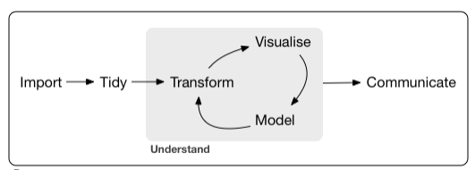
Resources
Data vizualization
Data vizualization
Graph purposes
Data vizualization
Graph purposes
- Analysis graphs
- design to see patterns, trends
- aid the process of data description
- interpretation
Data vizualization
Graph purposes
- Analysis graphs
- design to see patterns, trends
- aid the process of data description
- interpretation
- Presentation graphs
- design to attract attention
- make a point
- illustrate a conclusion
Source: Michael Friendly - http://datavis.ca/courses/RGraphics/
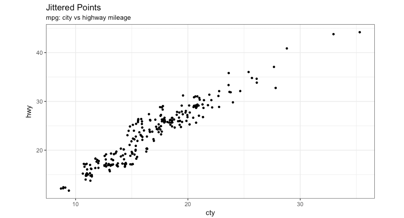
Graph types
Jitter
- Two variables numerical
Graph types
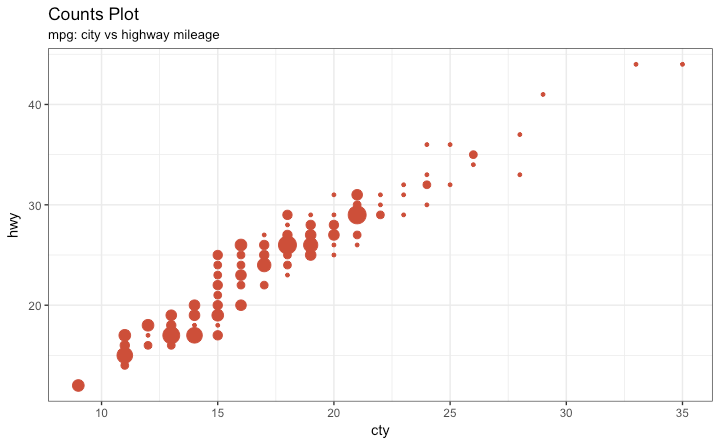
Bubble
- Two variables numerical
- Add another variable numerical
Graph types
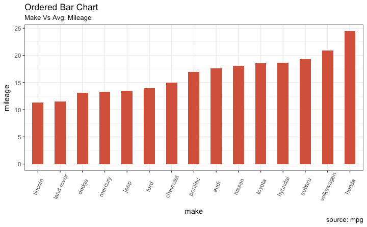
Bargraphs
- One variable categorical
- One variable numerical
Graph types
Bargraphs
- Rotate
Graph types
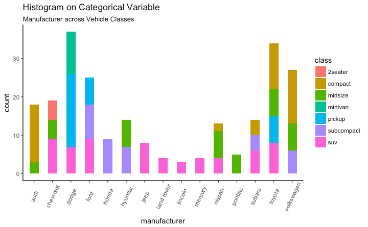
Bargraphs
- Two variable categorical
- One variable numerical
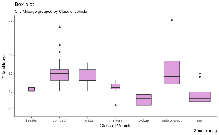
Graph types
Boxplots
- One variable categorical
- One variable numerical but with many values
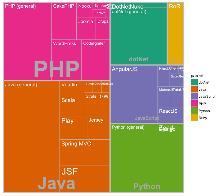
Graph types
Treemaps
- One variable categorical
- One variable numerical
- Much better than pie charts
ggplot2
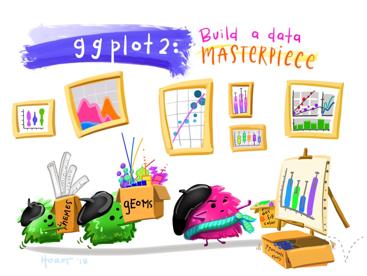
@allison_horst
ggplot2
A simple plot
- Choose the data set
- Choose the geometric representation
- Choose the aesthetics : x,y, color, shape etc...
ggplot(data=samples) + geom_point(mapping = aes(x=phosphates, y=nitrates))- All functions are from ggplot2 package unless specified

ggplot2
The grammar of graphics
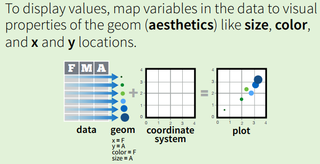
Every graph can be described as a combination of independent building blocks:
- data: a data frame: quantitative, categorical; local or data base query
- aesthetic mapping of variables into visual properties: size, color, x, y
- geometric objects (“geom”): points, lines, areas, arrows, …
- coordinate system (“coord”): Cartesian, log, polar, map
ggplot2
Syntax
ggplot(data=samples) + geom_point(mapping = aes(x=phosphates, y=nitrates))
ggplot2
Alternatively
ggplot(data=samples, mapping = aes(x=phosphates, y=nitrates)) + geom_point()- If different geometries origniate from different datasets or have different mapping the datasets or the mapping must be called inside the geom function.

ggplot2
Alternatively
ggplot(samples, aes(x=phosphates, y=nitrates)) + geom_point()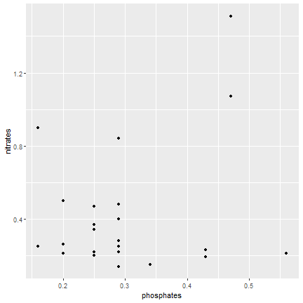
ggplot2
Make dot size bigger
ggplot(samples, aes(x=phosphates, y=nitrates))
ggplot2
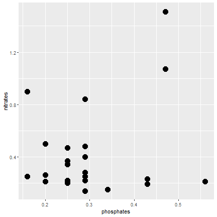
Make dot size bigger
ggplot(samples, aes(x=phosphates, y=nitrates)) + geom_point(size=5)- Add: size=5 outside of the aesthetics function
ggplot2
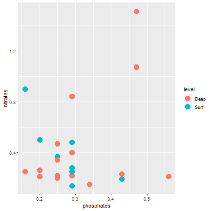
Color according to depth level (discrete)
ggplot(samples, aes(x=phosphates, y=nitrates, color=level)) + geom_point(size=5)- The mapping aesthetics must be an argument of the aes function
- geom_point(color=level, size=5) will generate an error...
ggplot2
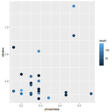
Color according to depth (continuous)
ggplot(samples, aes(x=phosphates, y=nitrates, color=depth)) + geom_point(size=5)- Add: color=depth
ggplot2
Symbol according to transect (continuous)
ggplot(samples, aes(x=phosphates, y=nitrates, color=depth, shape=transect)) + geom_point(size=5)- Add: shape=transect
Error: A continuous variable can not be mapped to shape
ggplot2
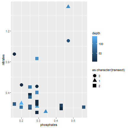
Symbol according to transect (continuous)
ggplot(samples, aes(x=phosphates, y=nitrates, color=depth, shape=as.character(transect))) + geom_point(size=5)- Add: shape=as.character(transect)
ggplot2
Panels depending on one variable
ggplot(samples, aes(x=phosphates, y=nitrates)) + geom_point() + facet_wrap(~ level)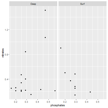
ggplot2
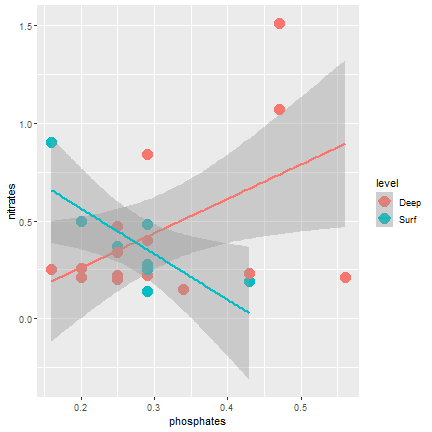
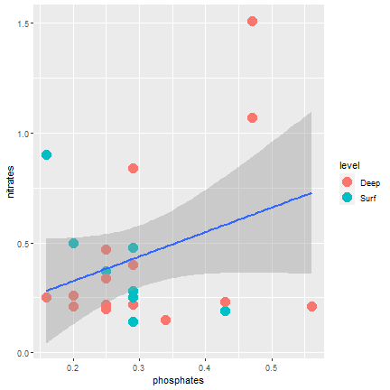
Adding a regression line
ggplot(samples, aes(x=phosphates, y=nitrates, color=level)) + geom_point(size=5) + geom_smooth(mapping = aes(x=phosphates, y=nitrates), method="lm")- Add: geom_smooth()
- You can choose the type of smoothing "lm" is for linear model
ggplot2
Adding a regression line
ggplot(samples, aes(x=phosphates, y=nitrates)) + geom_point(aes(color=level), size=5) + geom_smooth(mapping = aes(x=phosphates, y=nitrates), method="lm")- If the mapping is in the ggplot function is for all the geom....
ggplot2
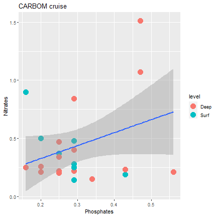
Finalizing the graph
ggplot(samples) + geom_point(mapping = aes(x=phosphates, y=nitrates, color=level), size=5) + geom_smooth(mapping = aes(x=phosphates, y=nitrates), method="lm") + xlab("Phosphates") + ylab("Nitrates") + ggtitle("CARBOM cruise")- Add: geom_smooth()
- You can choose the type of smoothing "lm" is for linear model
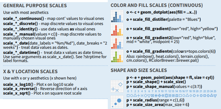
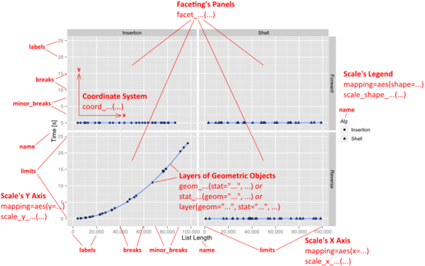
ggplot2 syntax
Anatomy of a plot
ggplot2 syntax
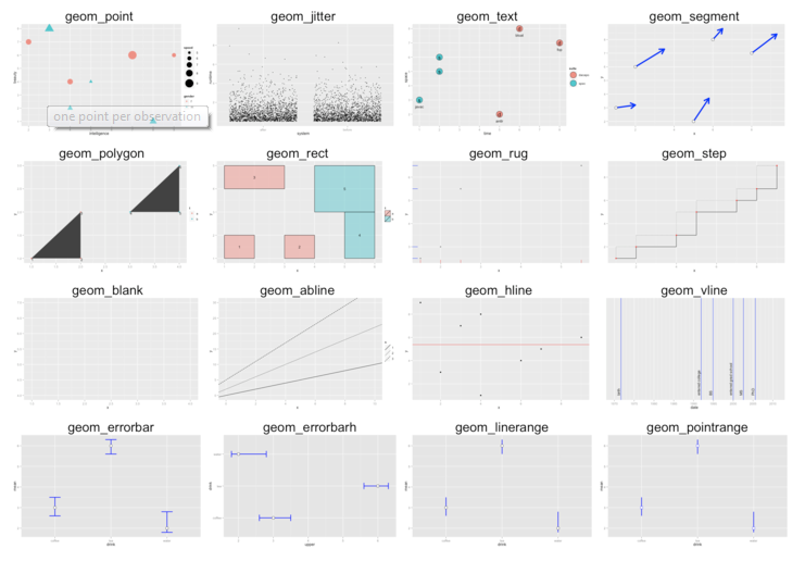
Geometries
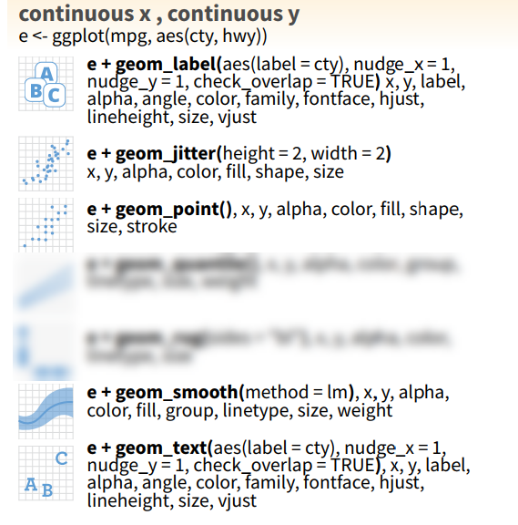
ggplot2 syntax
Continuous x and y
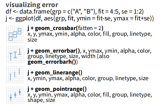
ggplot2 syntax
Plotting error
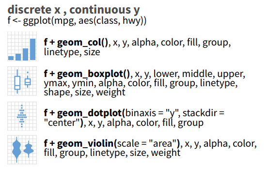
ggplot2 syntax
Discrete x - Continuous y
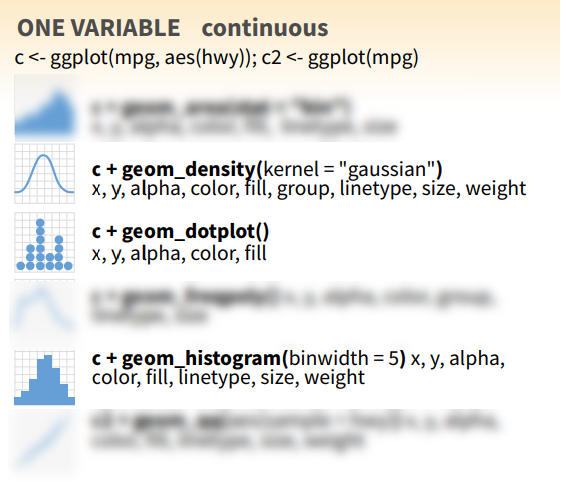
ggplot2 syntax
Continuous x
ggplot2 syntax
Modifying axis and scales