R course

Daniel Vaulot

2023-01-18

05 - Metabarcode processing with dada2

Introduction

This tutorial explain how to process Illumina data with the Dada2 suite as implemented in R (dada2 is also implemented in Qiime).

It is adapted from the Dada2 tutorial

Directory structure

Relative to the main directory from GitHub

• ../fastq : fastq files
• ../fastq_filtered : fastq files after filtration
• ../qual_pdf : qual pdf files
• ../dada2 : dada2 processed files
• ../databases : PR2 database file
• ../blast : BLAST files output
• ../R : This tutorial for Illumina files

Downloads

Install the following software :

• R

• R studio

Download and install the following libraries by running under R studio the following lines

install.packages("readr")     # To read and write files
install.packages("readxl")    # To read excel files

install.packages("dplyr")     # To manipulate dataframes
install.packages("tibble")    # To work with data frames
install.packages("tidyr")     # To work with data frames

install.packages("stringr")   # To manipulate strings

install.packages("ggplot2")   # To do plots


if (!requireNamespace("BiocManager", quietly = TRUE))
    install.packages("BiocManager")

BiocManager::install("Biobase")
BiocManager::install("Biostrings")
BiocManager::install("dada2")
BiocManager::install("phyloseq")

Data used

The samples originate from the CARBOM cruise (2013) off Brazil.

Samples have been sorted by flow cytometry and 3 genes have been PCR amplified :

• 18S rRNA - V4 region
• 16S rNA with plastid
• nifH

The PCR products have been sequenced by 1 run of Illumina 2*250 bp. The data consist of the picoplankton samples from one transect and fastq files have been subsampled with 1000 sequences per sample.

References

• Gerikas Ribeiro C, Marie D, Lopes dos Santos A, Pereira Brandini F, Vaulot D. (2016). Estimating microbial populations by flow cytometry: Comparison between instruments. Limnol Oceanogr Methods 14:750–758.
• Gerikas Ribeiro C, Lopes dos Santos A, Marie D, Brandini P, Vaulot D. (2018). Relationships between photosynthetic eukaryotes and nitrogen-fixing cyanobacteria off Brazil. ISME J in press.
• Gerikas Ribeiro C, Lopes dos Santos A, Marie D, Helena Pellizari V, Pereira Brandini F, Vaulot D. (2016). Pico and nanoplankton abundance and carbon stocks along the Brazilian Bight. PeerJ 4:e2587.

Set-up

Load the necessary libraries

  library("dada2")
  library("phyloseq") 
  library("Biostrings")
  
  library("ggplot2")

  library("dplyr")
  library("tidyr")
  library("tibble")

  library("readxl")
  library("readr")

  library("stringr")

  library("kableExtra") # necessary for nice table formatting with knitr

Set up directories

Create directories that will be used to stored the files at the different stage of the processing

# change the following line to the path where you unzipped the tutorials


  fastq_dir <-    "../fastq/"           # fastq directory
  filtered_dir <- "../fastq_filtered/"  # fastq filtered
  qual_dir <-     "../qual_pdf/"        # qual pdf
  dada2_dir <-    "../dada2/"           # dada2 results
  blast_dir <-    "../blast/"           # blast2 results
  database_dir <- "../databases/"       # databases
  
  dir.create(filtered_dir)
  dir.create(qual_dir)
  dir.create(dada2_dir)
  dir.create(blast_dir)

Setup variables

Primers

Note that the primers are degenerated.

Dada2 has an option to remove primers (FilterandTrim) but this function will not accept degeneracy.

  primer_set_fwd = c("CCAGCAGCCGCGGTAATTCC", "CCAGCACCCGCGGTAATTCC", 
                     "CCAGCAGCTGCGGTAATTCC", "CCAGCACCTGCGGTAATTCC")
  primer_set_rev = c("ACTTTCGTTCTTGATYRATGA")
  primer_length_fwd <- str_length(primer_set_fwd[1]) 
  primer_length_rev <- str_length(primer_set_rev[1])

PR2 tax levels

  PR2_tax_levels <- c("Kingdom", "Supergroup","Division", "Class", 
                      "Order", "Family", "Genus", "Species")

Examine the fastQ files

Construct a list of the fastq files

It is assumed that the sample names are at the start of file name and separated by _.

# get a list of all fastq files in the ngs directory and separate R1 and R2
  fns <- sort(list.files(fastq_dir, full.names = TRUE)) 
  fns <- fns[str_detect( basename(fns),".fastq")]
  fns_R1 <- fns[str_detect( basename(fns),"R1")]
  fns_R2 <- fns[str_detect( basename(fns),"R2")]

# Extract sample names, assuming filenames have format: SAMPLENAME_XXX.fastq
  sample.names <- str_split(basename(fns_R1), pattern = "_", simplify = TRUE) 
  sample.names <- sample.names[,1]
  sample.names

 [1] "120p" "121p" "122p" "125p" "126p" "140p" "141p" "142p" "155p" "156p"
[11] "157p" "165p" "166p" "167p"

Compute number of paired reads

# create an empty data frame  
  df <- data.frame()  

# loop through all the R1 files (no need to go through R2 which should be the same) 

  for(i in 1:length(fns_R1)) { 
    # use the dada2 function fastq.geometry
      geom <- fastq.geometry(fns_R1[i])
    # extract the information on number of sequences and file name 
      df_one_row <- data.frame (n_seq=geom[1], file_name=basename(fns_R1[i]) )
    # add one line to data frame
      df <- bind_rows(df, df_one_row)
  } 

Display results

# display number of sequences
  DT::datatable(df)

# plot the histogram with number of sequences
  g <- ggplot(df, aes(x=n_seq)) + 
        geom_histogram( alpha = 0.5, position="identity", binwidth = 10) +
        xlim(0, 2000)
  
  print(g)

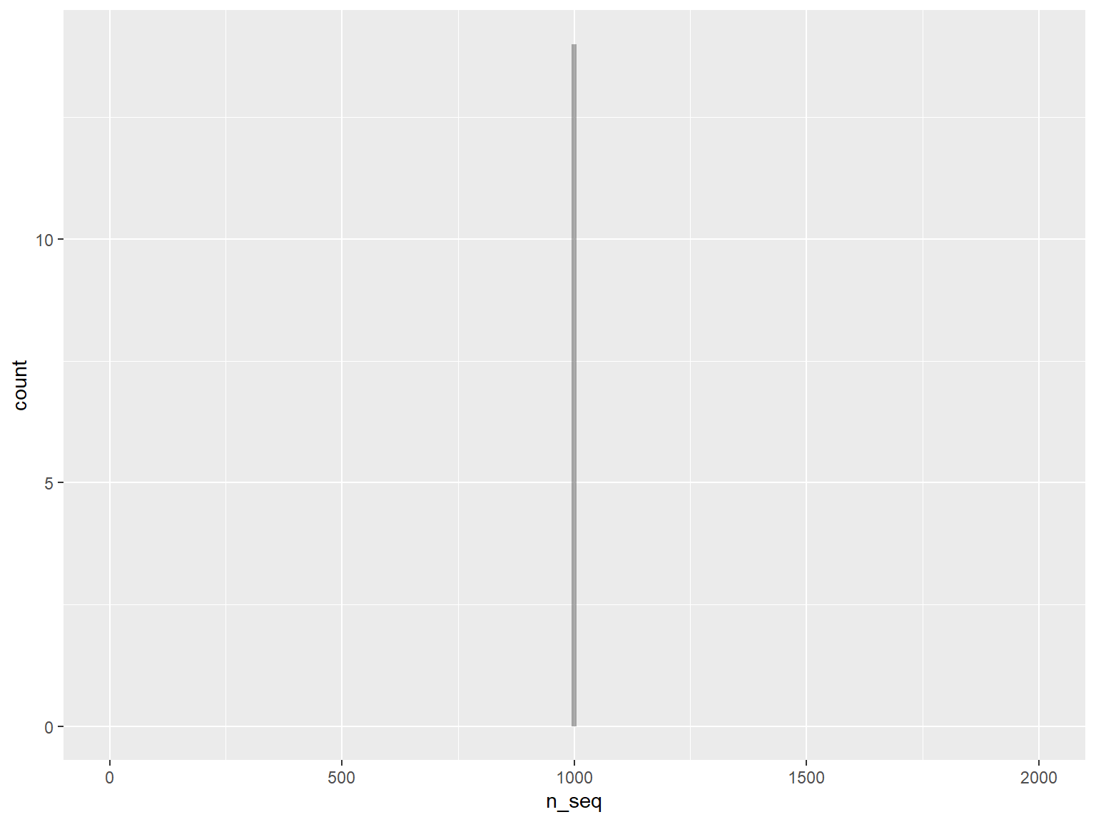
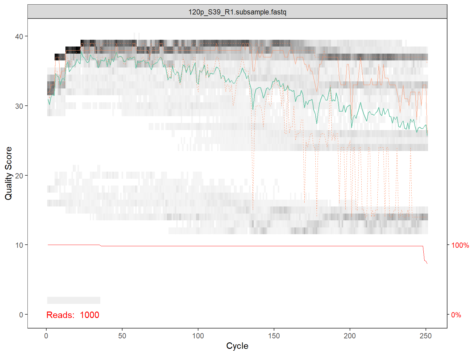
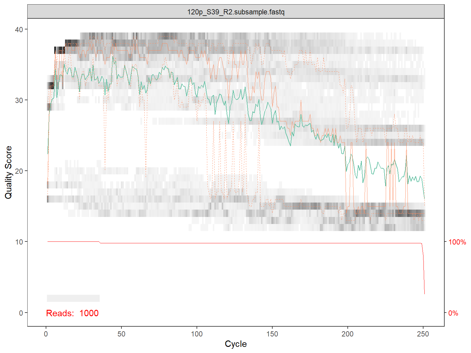
Plot quality for reads

 for(i in 1:length(fns)) { 
   
  # Use dada2 function to plot quality
    p1 <- plotQualityProfile(fns[i])
    
  # Only plot on screen for first 2 files  
    if (i <= 2) {print(p1)}
    
  # save the file as a pdf file (uncomment to execute)
    p1_file <- paste0(qual_dir, basename(fns[i]),".qual.pdf")
    ggsave( plot=p1, filename= p1_file,
              device = "pdf", width = 15, height = 15, scale=1, units="cm")
  }   

Filter and Trim the reads

Two approaches

The dada2 algorithm requires primers to be removed prior to processing.

• Using dada2 there are 2 possibilities
  • Remove by sequence, but dada2 does not allow for ambiguities
  • Remove by position, which is not a problem for Illumina sequences but is a problem for 454
• For complex situation we recommend to use cutadapt to remove the primers.

Create names for the filtered files

We create the name of the files that will be generated by the filterAndTrim function in the step below.

These names are composed by the path name (“../fastq_filtered/”), the sample names, the read number (R1 or R2) and a “_filt” suffix.

  filt_R1 <- str_c(filtered_dir, sample.names, "_R1_filt.fastq")
  filt_R2 <- str_c(filtered_dir, sample.names, "_R2_filt.fastq")

Method 1 - Removing the primers by sequence

(DO NOT EXECUTE THIS STEP)

The next piece of code could be used to remove the primers by sequence.

The dada2 package does not allow for primer degeneracy. Since our forward primer is degenerated at two positions, all four combinations need to be tested.

However it will be necessary to re-assemble after that the 4 fastQ files created (which has not to done).

So the better strategy is to remove primer by truncation (see next step).

# On Windows set multithread=FALSE  

  out_all <-data.frame(id=length(fns_R1))
  for (i in 1:4) {
    out <- filterAndTrim(fns_R1, filt_R1, fns_R2, filt_R2, truncLen=c(250,240), trimLeft = c(0,0),
              maxN=0, maxEE=c(Inf, Inf), truncQ=10, rm.phix=TRUE, primer.fwd = primer_set_fwd[i], 
              compress=FALSE, multithread=FALSE) 
    out_all <- cbind(out_all, out)

  }

  knitr::kable(out_all)

Method 2 - Remove primers by truncation and filter

Filter all sequences with N, truncate R2 to 240 bp

  out <- filterAndTrim(fns_R1, filt_R1, fns_R2, filt_R2, 
                       truncLen=c(250,240), trimLeft = c(primer_length_fwd,primer_length_rev),
                       maxN=0, maxEE=c(2, 2), truncQ=10, rm.phix=TRUE,  
                       compress=FALSE, multithread=FALSE) 
  knitr::kable(out)

	reads.in	reads.out
120p_S39_R1.subsample.fastq	1000	256
121p_S57_R1.subsample.fastq	1000	457
122p_S4_R1.subsample.fastq	1000	407
125p_S22_R1.subsample.fastq	1000	553
126p_S40_R1.subsample.fastq	1000	508
140p_S5_R1.subsample.fastq	1000	456
141p_S23_R1.subsample.fastq	1000	473
142p_S41_R1.subsample.fastq	1000	583
155p_S59_R1.subsample.fastq	1000	528
156p_S6_R1.subsample.fastq	1000	530
157p_S24_R1.subsample.fastq	1000	513
165p_S42_R1.subsample.fastq	1000	521
166p_S60_R1.subsample.fastq	1000	519
167p_S7_R1.subsample.fastq	1000	572

Dada2 processing

Learn error rates

The error rates are plotted.

R1

  err_R1 <- learnErrors(filt_R1, multithread=FALSE)

  plotErrors(err_R1, nominalQ=TRUE)

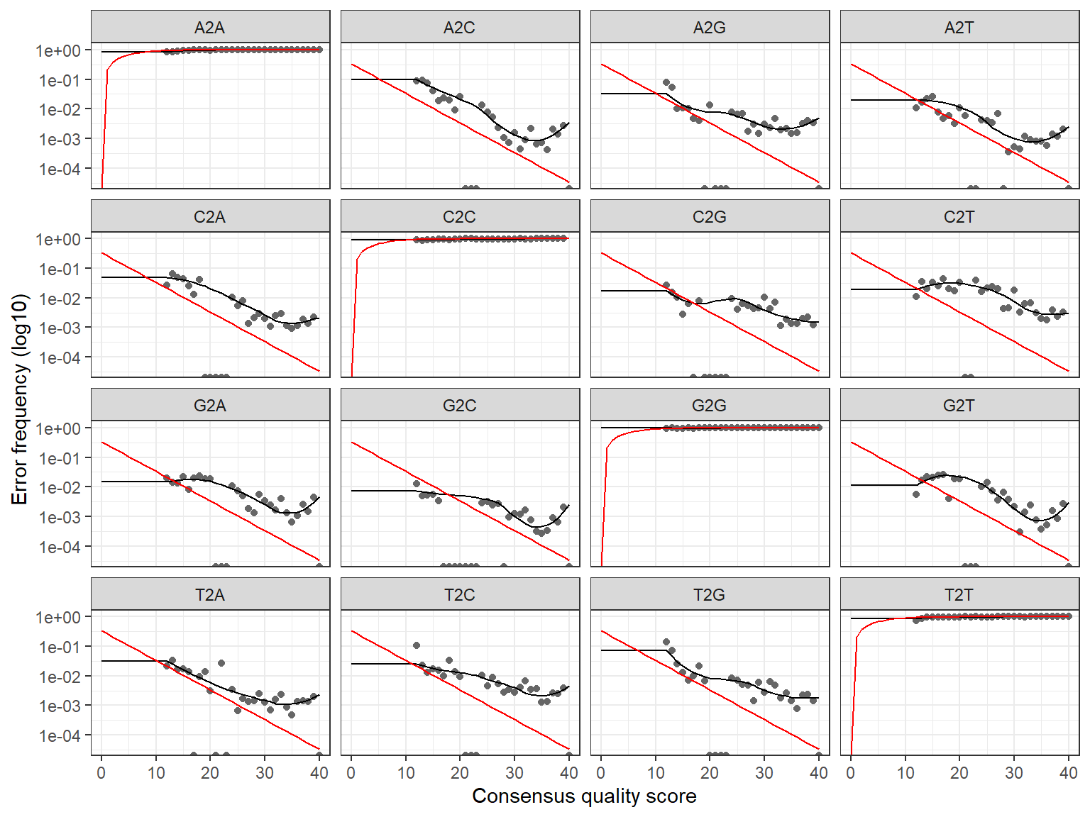
1581480 total bases in 6876 reads from 14 samples will be used for learning the error rates.

R2

  err_R2 <- learnErrors(filt_R2, multithread=FALSE)

  plotErrors(err_R2, nominalQ=TRUE)

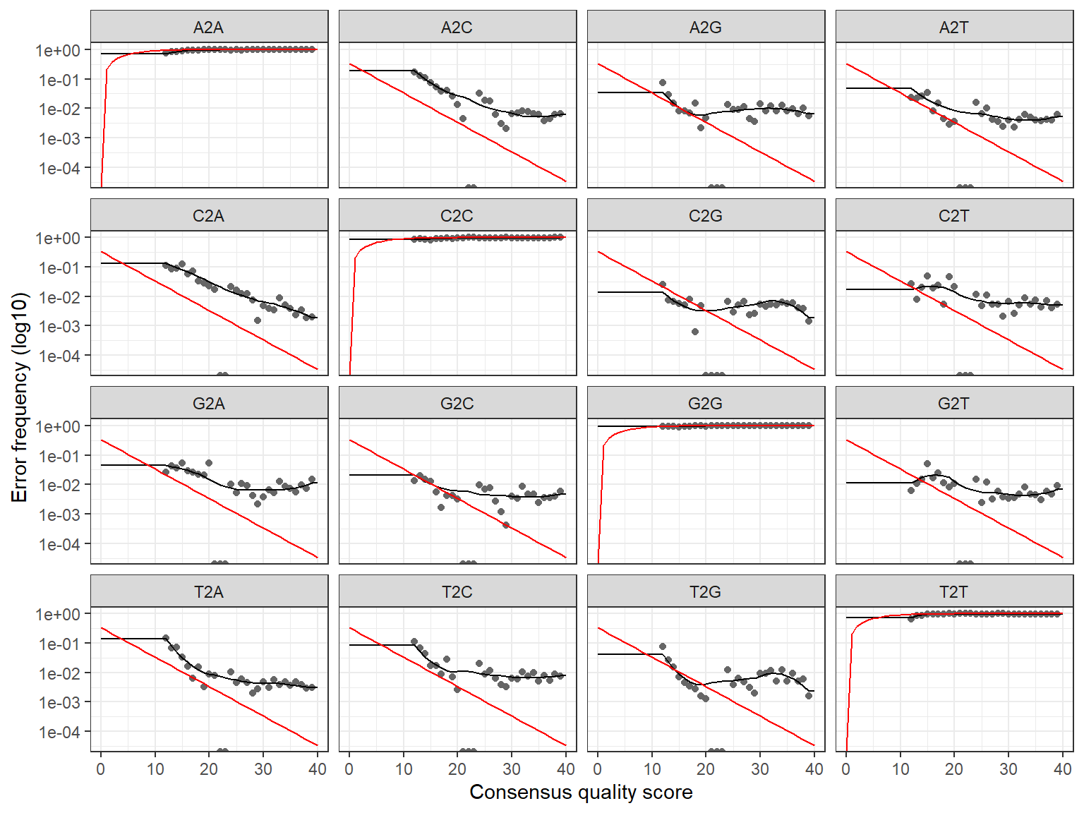
1505844 total bases in 6876 reads from 14 samples will be used for learning the error rates.

Dereplicate the reads

R1

  derep_R1 <- derepFastq(filt_R1, verbose=FALSE)
  
# Name the derep-class objects by the sample names
  names(derep_R1) <- sample.names

R2

  derep_R2 <- derepFastq(filt_R2, verbose=FALSE)
  
# Name the derep-class objects by the sample names
  names(derep_R2) <- sample.names 

Sequence-variant inference algorithm to the dereplicated data

R1

    dada_R1 <- dada(derep_R1, err=err_R1, multithread=FALSE, pool=FALSE)
    
    dada_R1[[1]]

Sample 1 - 256 reads in 93 unique sequences.
Sample 2 - 457 reads in 166 unique sequences.
Sample 3 - 407 reads in 128 unique sequences.
Sample 4 - 553 reads in 220 unique sequences.
Sample 5 - 508 reads in 219 unique sequences.
Sample 6 - 456 reads in 147 unique sequences.
Sample 7 - 473 reads in 180 unique sequences.
Sample 8 - 583 reads in 211 unique sequences.
Sample 9 - 528 reads in 172 unique sequences.
Sample 10 - 530 reads in 211 unique sequences.
Sample 11 - 513 reads in 177 unique sequences.
Sample 12 - 521 reads in 199 unique sequences.
Sample 13 - 519 reads in 172 unique sequences.
Sample 14 - 572 reads in 170 unique sequences.
dada-class: object describing DADA2 denoising results
5 sequence variants were inferred from 93 input unique sequences.
Key parameters: OMEGA_A = 1e-40, OMEGA_C = 1e-40, BAND_SIZE = 16

R2

    dada_R2 <- dada(derep_R2, err=err_R2, multithread=FALSE, pool=FALSE)
    
    dada_R2[[1]]

Sample 1 - 256 reads in 236 unique sequences.
Sample 2 - 457 reads in 391 unique sequences.
Sample 3 - 407 reads in 299 unique sequences.
Sample 4 - 553 reads in 409 unique sequences.
Sample 5 - 508 reads in 451 unique sequences.
Sample 6 - 456 reads in 335 unique sequences.
Sample 7 - 473 reads in 347 unique sequences.
Sample 8 - 583 reads in 458 unique sequences.
Sample 9 - 528 reads in 418 unique sequences.
Sample 10 - 530 reads in 404 unique sequences.
Sample 11 - 513 reads in 384 unique sequences.
Sample 12 - 521 reads in 395 unique sequences.
Sample 13 - 519 reads in 396 unique sequences.
Sample 14 - 572 reads in 400 unique sequences.
dada-class: object describing DADA2 denoising results
3 sequence variants were inferred from 236 input unique sequences.
Key parameters: OMEGA_A = 1e-40, OMEGA_C = 1e-40, BAND_SIZE = 16

Merge sequences

    mergers <- mergePairs(dada_R1, derep_R1, dada_R2, derep_R2, verbose=TRUE)
    
  # Inspect the merger data.frame from the first sample

  df_table <- mergers[[1]] %>% 
    mutate(sequence = str_c(str_sub(sequence, 1, 20), "..."))

  kable(df_table, "html")

sequence	abundance	forward	reverse	nmatch	nmismatch	nindel	prefer	accept
AGCTCCAATAGCGTATATTA...	146	1	1	71	0	0	1	TRUE
CACACGTCTAATGTTGCATT...	64	2	2	131	0	0	1	TRUE
AGCTCCAATAGCGTATACTA...	13	3	3	72	0	0	1	TRUE

Make sequence table

    seqtab <- makeSequenceTable(mergers)
    
    dim(seqtab)
    
  # Make a transposed of the seqtab to make it be similar to mothur database
    t_seqtab <- t(seqtab)

  # Inspect distribution of sequence lengths
    table(nchar(getSequences(seqtab))) 

[1] 14 58

318 351 360 363 367 369 371 372 373 375 376 377 378 379 380 382 383 384 387 388 
  3   1   1   3   1   1   2   1   2   1   3   6  12   4   4   2   5   2   1   3 

Remove chimeras

Note that remove chimeras will produce spurious results if primers have not be removed. The parameter methods can be pooled or consensus

    seqtab.nochim <- removeBimeraDenovo(seqtab, method="consensus", multithread=FALSE, verbose=TRUE)

  # Compute % of non chimeras
    paste0("% of non chimeras : ",sum(seqtab.nochim)/sum(seqtab)*100)
    paste0("total number of sequences : ",sum(seqtab.nochim))

[1] "% of non chimeras : 100"
[1] "total number of sequences : 5868"

In our case there were no chimeras found. It is noteworthy that the total number of sequences is almost twice that what is recovered with mothur which is 2573

Track number of reads at each step

  # define a function
    getN <- function(x) sum(getUniques(x))
    
    track <- cbind(out, sapply(dada_R1, getN), sapply(mergers, getN), 
                   rowSums(seqtab), rowSums(seqtab.nochim))

    colnames(track) <- c("input", "filtered", "denoised", "merged", "tabled", "nonchim")
    rownames(track) <- sample.names
    
    knitr::kable(track)  
    write_tsv(data.frame(track), str_c(dada2_dir,"read_numbers_dada2.tsv"))

	input	filtered	denoised	merged	tabled	nonchim
120p	1000	256	241	223	223	223
121p	1000	457	446	397	397	397
122p	1000	407	396	357	357	357
125p	1000	553	551	464	464	464
126p	1000	508	493	340	340	340
140p	1000	456	441	427	427	427
141p	1000	473	460	381	381	381
142p	1000	583	567	495	495	495
155p	1000	528	524	445	445	445
156p	1000	530	525	425	425	425
157p	1000	513	507	438	438	438
165p	1000	521	509	442	442	442
166p	1000	519	510	478	478	478
167p	1000	572	563	556	556	556

Transforming and saving the ASVs sequences

In the output of dada2, otu names are the sequences.

We change to give a Otuxxx name and the sequences are stored in the taxonomy table.

  seqtab.nochim_trans <- as.data.frame(t(seqtab.nochim)) %>% 
    rownames_to_column(var = "sequence") %>%
    rowid_to_column(var = "OTUNumber") %>% 
    tibble::remove_rownames() %>%
    mutate(OTUNumber = sprintf("otu%04d", OTUNumber)) %>% 
    mutate(sequence = str_replace_all(sequence, "(-|\\.)",""))

  df <- seqtab.nochim_trans
  seq_out <- Biostrings::DNAStringSet(df$sequence)

  names(seq_out) <- df$OTUNumber

  Biostrings::writeXStringSet(seq_out, str_c(dada2_dir, "CARBOM_ASV_no_taxo.fasta"), 
                              compress=FALSE, width = 20000)

Assigning taxonomy

This step is quite long… If you want to skip please go to next step.

    pr2_file <- paste0(database_dir, "pr2_version_4.14.0_SSU_dada2.fasta.gz")
    taxa <- assignTaxonomy(seqtab.nochim, refFasta=pr2_file,  
                           taxLevels = PR2_tax_levels,
                           minBoot = 0, outputBootstraps = TRUE,
                           verbose = TRUE)
    saveRDS(taxa, str_c(dada2_dir, "CARBOM.taxa.rds"))

Export data

Export

We need to reformat the data produced by dada2 if we want to use for further analysis, for example with Phyloseq or BLAST.

Export data as produced by Dada2

  taxa <-  readRDS(str_c(dada2_dir, "CARBOM.taxa.rds"))  
  write_tsv(as.tibble(taxa$tax), path = str_c(dada2_dir, "taxa.txt"))  
  write_tsv(as.tibble(taxa$boot), path = str_c(dada2_dir, "taxa_boot.txt"))
  write_tsv(as.tibble(seqtab.nochim), path = str_c(dada2_dir, "seqtab.txt"))

Appending taxonomy and boot to the sequence table

    taxa_tax <- as.data.frame(taxa$tax)
    taxa_boot <- as.data.frame(taxa$boot) %>% 
      rename_all(funs(str_c(.,"_boot")))
    seqtab.nochim_trans <- seqtab.nochim_trans %>% 
      bind_cols(taxa_tax) %>% 
      bind_cols(taxa_boot)

Filter for 18S

Remember that we sequenced 3 genes (18S, 16S plastid and nifH).

We remove the sequences that are not 18S by selecting only bootstrap values for Supergroup in excess of 80.

    bootstrap_min <- 80

  # Filter based on the bootstrap
    seqtab.nochim_18S <- seqtab.nochim_trans %>%  
      dplyr::filter(Supergroup_boot >= bootstrap_min) 
  
  # Create a database like file for dada2
    write_tsv(seqtab.nochim_18S, str_c(dada2_dir, "CARBOM_dada2.database.tsv"))
    
    cat("Before filtration - # of sequences: ", nrow(seqtab.nochim_trans), "\n")
    cat("After filtration - # of sequences: ", nrow(seqtab.nochim_18S), "\n")

Before filtration - # of sequences:  58 
After filtration - # of sequences:  53 

Write FASTA file for BLAST analysis with taxonomy

Use the Biostrings library

  df <- seqtab.nochim_18S
  seq_out <- Biostrings::DNAStringSet(df$sequence)

  names(seq_out) <- str_c(df$OTUNumber,
                                df$Supergroup,
                                df$Division,
                                df$Class,
                                df$Order,
                                df$Family,
                                df$Genus,
                                df$Species,
                                sep="|")

  Biostrings::writeXStringSet(seq_out, str_c(blast_dir, "CARBOM_ASV.fasta"), 
                              compress=FALSE, width = 20000)

Write FASTA file for BLAST analysis with taxonomy

This file can be sent to a server and a BLAST analysis can be done using the following bash file

#!/bin/bash

# Replace the next line by the location of the directory where you have your data
DIR_PROJECT="/projet/sbr/ccebarcodep1408/workshop_nz_2018/blast/"

cd $DIR_PROJECT

FILE="CARBOM_ASV"

FASTA=$DIR_PROJECT$FILE".fasta"
BLAST_TSV=$DIR_PROJECT$FILE".blast.tsv"

OUT_FMT="6 qseqid sseqid sacc stitle sscinames staxids sskingdoms sblastnames pident slen length mismatch gapopen qstart qend sstart send evalue bitscore"

blastn -max_target_seqs 100 -evalue 1.00e-10 -query $FASTA -out $BLAST_TSV -db /db/blast/all/nt -outfmt "$OUT_FMT"

Phyloseq

Create and save a phyloseq object from dada2 results

samdf <- data.frame(sample_name=sample.names)
rownames(samdf) <- sample.names

OTU <- seqtab.nochim_18S %>% 
    tibble::remove_rownames() %>% 
    tibble::column_to_rownames("OTUNumber") %>% 
    select_if(is.numeric) %>% 
    select(-contains("_boot")) %>% 
    as.matrix() %>% 
    otu_table(taxa_are_rows=TRUE) 
    
TAX <- seqtab.nochim_18S %>% 
  tibble::remove_rownames()%>% 
  tibble::column_to_rownames("OTUNumber") %>%
  select(Kingdom:Species)%>% 
  as.matrix() %>%  
  tax_table()

ps_dada2 <- phyloseq(OTU, 
               sample_data(samdf), 
               TAX)
saveRDS(ps_dada2,str_c(dada2_dir, "CARBOM_phyloseq.rds"))