R course

Daniel Vaulot

2023-01-26

Metabarcode analysis - Phyloseq

R - Phyloseq

• Introduction to the data
• Read the data
• Format and save as Phyloseq objects
• Filter data
• Bar graphs
• Alpha diversity
• Beta diversity

Phyloseq R library

• Phyloseq web site

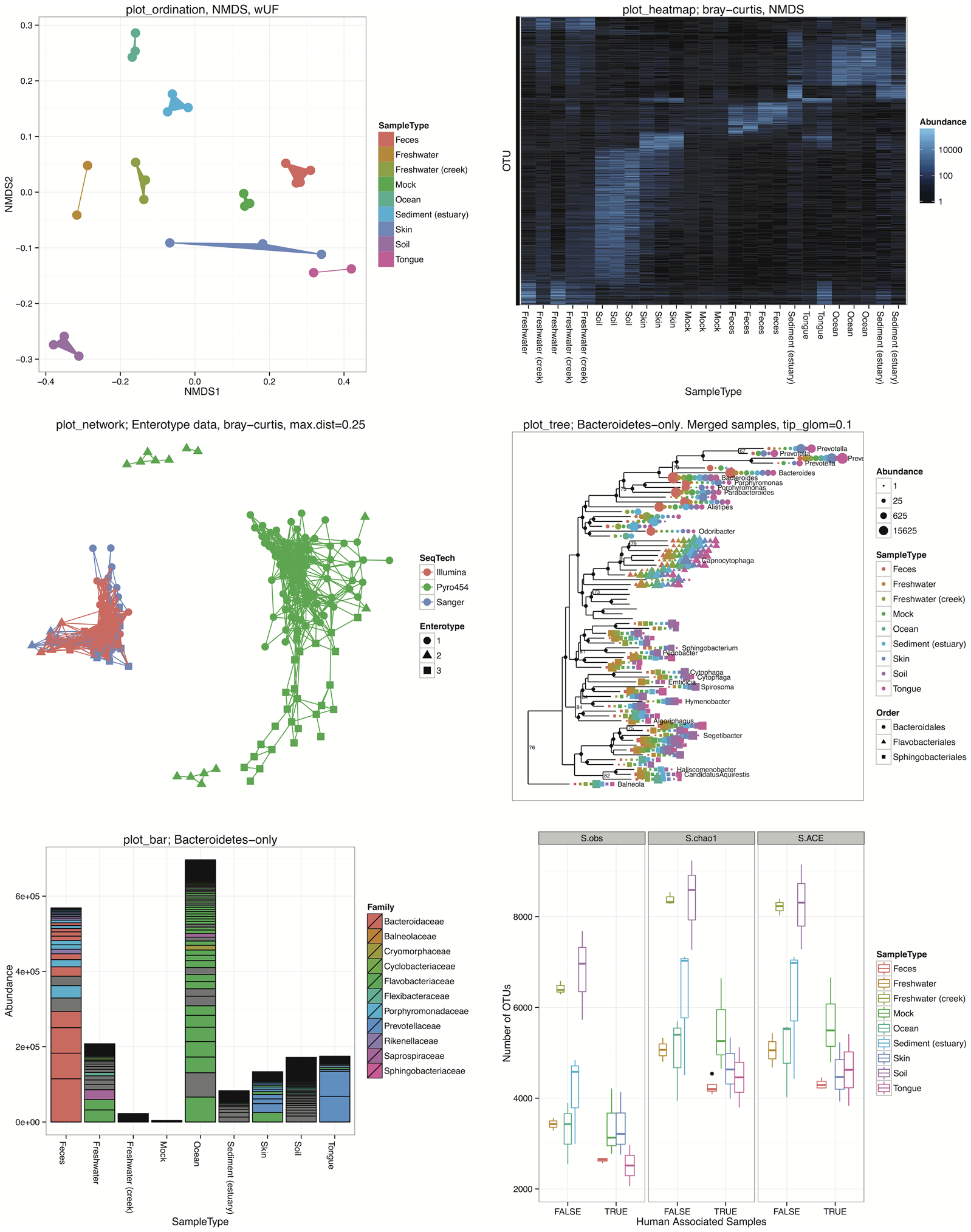
• See in particular tutorials for

  • importing data

  • bar plots

• Get ASVs, read abundance and metadata all together

• Filter and regroup the data

• Bar plots, Alpha and Beta diversity computations

Data

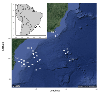
This tutorial uses a reduced metabarcoding dataset obtained by C. Ribeiro and A. Lopes dos Santos. This dataset originates from the CARBOM cruise in 2013 off Brazil and corresponds to the 18S V4 region amplified on flow cytometry sorted samples (see pptx file for details) and sequenced on an Illumina run 2*250 bp analyzed with mothur.

Reference

• Gérikas Ribeiro, C., Dos Santos, A.L., Marie, D., Brandini, F.P. & Vaulot, D. 2018. Small eukaryotic phytoplankton communities in tropical waters off Brazil are dominated by symbioses between Haptophyta and nitrogen-fixing cyanobacteria. ISME Journal. 12:1360–74.

Libraries

library("phyloseq")
library("ggplot2")      # graphics
library("readxl")       # necessary to import the data from Excel file
library("dplyr")        # filter and reformat data frames
library("tibble")       # Needed for converting column to row names

Import and format data

Three tables are needed

• OTU
• Taxonomy
• Samples

They are read from a single Excel file where each sheet contains one of the tables

OTU

• rows = OTUs or ASVs
• cols = samples
• cells = number of reads

Table OTU - OTU abundance

Taxonomy

• rows = OTUs or ASVs
• cols = taxonomy ranks
• cells = taxon name

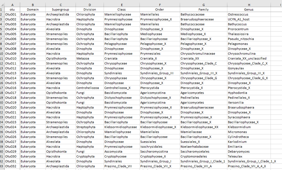
Table Taxo - OTU taxonomy

Samples

• rows = samples
• cols = metadata type
• cells = metadata values

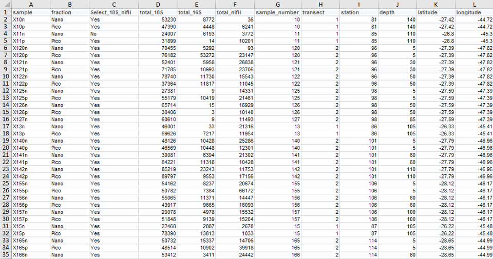
Table Samples

Read Excel files

  otu_mat<- read_excel("data/CARBOM metabarcodes.xlsx", sheet = "OTU matrix")

  tax_mat<- read_excel("data/CARBOM metabarcodes.xlsx", sheet = "Taxonomy table")

  samples_df <- read_excel("data/CARBOM metabarcodes.xlsx", sheet = "Samples")

Phyloseq objects need to have row.names

• define the row names from the otu column

  otu_mat <- otu_mat %>%
    tibble::column_to_rownames("otu") 

• Idem for the two other matrixes

  tax_mat <- tax_mat %>% 
    tibble::column_to_rownames("otu")

  samples_df <- samples_df %>% 
    tibble::column_to_rownames("sample") 

Transform to matrixes

Sample table can be left as data frame

  otu_mat <- as.matrix(otu_mat)

  tax_mat <- as.matrix(tax_mat)

Transform to phyloseq objects

  OTU = otu_table(otu_mat, taxa_are_rows = TRUE)

  TAX = tax_table(tax_mat)

  samples = sample_data(samples_df)
  
  carbom <- phyloseq(OTU, TAX, samples)

  carbom

phyloseq-class experiment-level object
otu_table()   OTU Table:         [ 287 taxa and 55 samples ]
sample_data() Sample Data:       [ 55 samples by 27 sample variables ]
tax_table()   Taxonomy Table:    [ 287 taxa by 7 taxonomic ranks ]

Check data

  sample_names(carbom)

 [1] "X10n"   "X10p"   "X11n"   "X11p"   "X120n"  "X120p"  "X121n"  "X121p" 
 [9] "X122n"  "X122p"  "X125n"  "X125p"  "X126n"  "X126p"  "X127n"  "X13n"  
[17] "X13p"   "X140n"  "X140p"  "X141n"  "X141p"  "X142n"  "X142p"  "X155n" 
[25] "X155p"  "X156n"  "X156p"  "X157n"  "X157p"  "X15n"   "X15p"   "X165n" 
[33] "X165p"  "X166n"  "X166p"  "X167n"  "X167p"  "X1n"    "X1p"    "X2n"   
[41] "X2p"    "X3n"    "X3p"    "X5n"    "X5p"    "X7n"    "X7p"    "X9n"   
[49] "X9p"    "tri01n" "tri01p" "tri02n" "tri02p" "tri03n" "tri03p"

  rank_names(carbom)

[1] "Domain"     "Supergroup" "Division"   "Class"      "Order"     
[6] "Family"     "Genus"     

  sample_variables(carbom)

 [1] "fraction"          "Select_18S_nifH"   "total_18S"        
 [4] "total_16S"         "total_nifH"        "sample_number"    
 [7] "transect"          "station"           "depth"            
[10] "latitude"          "longitude"         "picoeuks"         
[13] "nanoeuks"          "bottom_depth"      "level"            
[16] "transect_distance" "date"              "time"             
[19] "phosphates"        "silicates"         "ammonia"          
[22] "nitrates"          "nitrites"          "temperature"      
[25] "fluorescence"      "salinity"          "sample_label"     

Filter and normalize data

Keep only samples to be analyzed

  carbom <- subset_samples(carbom, Select_18S_nifH =="Yes")
  
  carbom

phyloseq-class experiment-level object
otu_table()   OTU Table:         [ 287 taxa and 54 samples ]
sample_data() Sample Data:       [ 54 samples by 27 sample variables ]
tax_table()   Taxonomy Table:    [ 287 taxa by 7 taxonomic ranks ]

Keep only photosynthetic taxa

  carbom <- subset_taxa(carbom, Division %in% c("Chlorophyta", "Dinophyta", "Cryptophyta", 
                                                "Haptophyta", "Ochrophyta", "Cercozoa"))

  carbom <- subset_taxa(carbom, !(Class %in% c("Syndiniales", "Sarcomonadea")))

  carbom

phyloseq-class experiment-level object
otu_table()   OTU Table:         [ 205 taxa and 54 samples ]
sample_data() Sample Data:       [ 54 samples by 27 sample variables ]
tax_table()   Taxonomy Table:    [ 205 taxa by 7 taxonomic ranks ]

Normalize

Normalize number of reads in each sample using median number of reads.

  total = median(sample_sums(carbom))

  standf = function(x, t=total) round(t * (x / sum(x)))

  carbom = transform_sample_counts(carbom, standf)

The number of reads used for normalization is 44903.

Bar graphs

Basic bar graph based on Division

plot_bar(carbom, fill = "Division")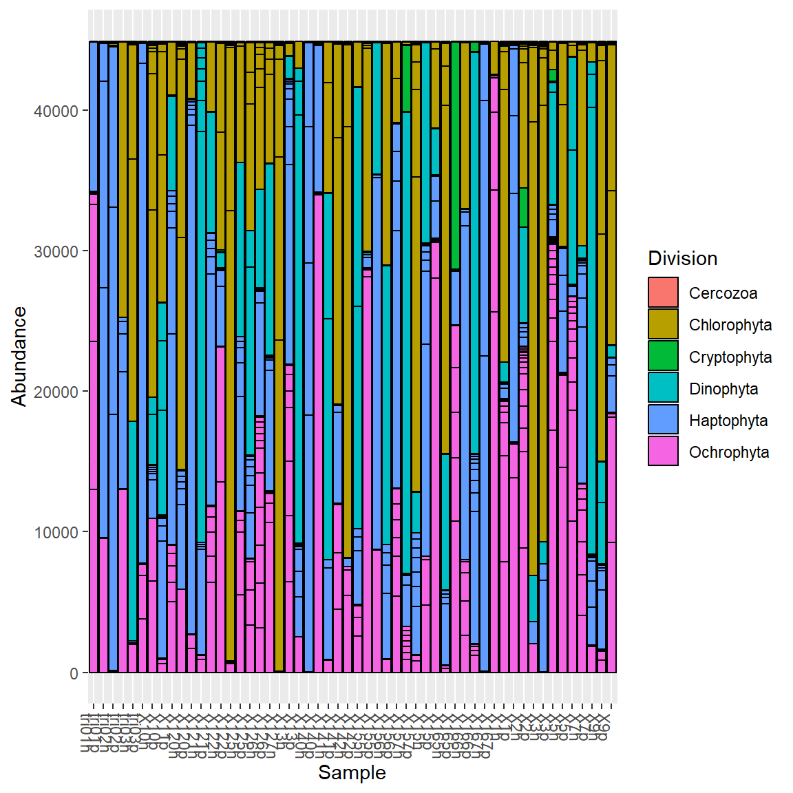

Remove OTUs boundaries.

# This is done by adding ggplot2 modifier.

plot_bar(carbom, fill = "Division") + 
 geom_bar(aes(color=Division, 
              fill=Division), 
          stat="identity", 
          position="stack")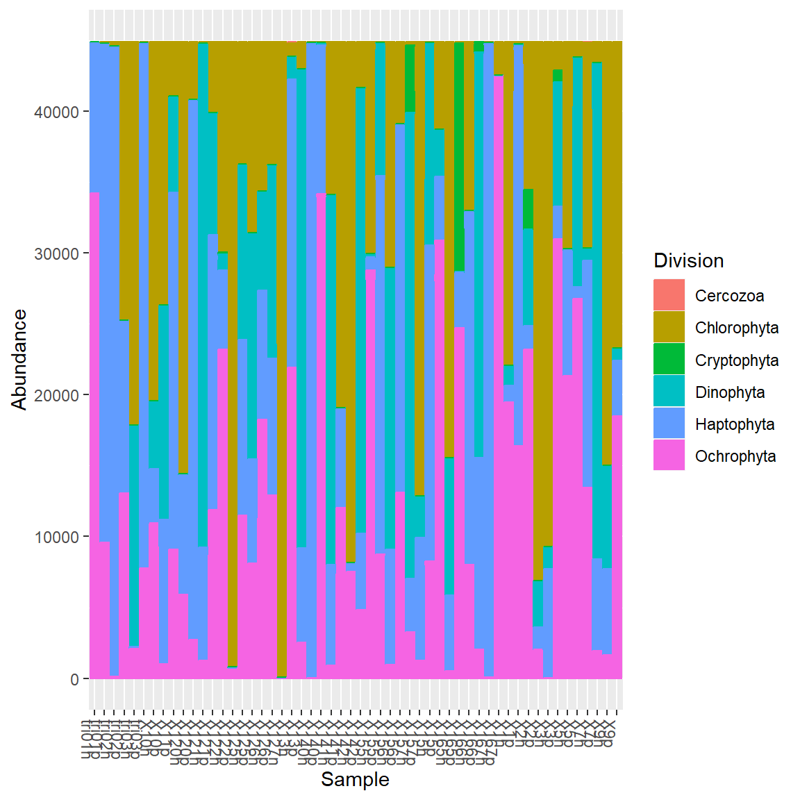

Group together Pico vs Nano samples.

carbom_fraction <- merge_samples(carbom, "fraction")

plot_bar(carbom_fraction, fill = "Division") + 
  geom_bar(aes(color=Division, 
               fill=Division), 
           stat="identity", 
           position="stack")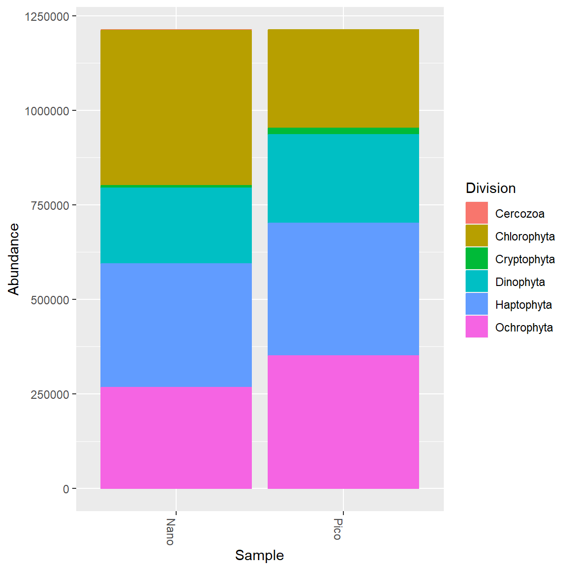

More grouping

# Keep only Chlorophyta
# Color according to genus. 
# Pico vs Nano/Surface vs Deep.

  carbom_chloro_ps <- subset_taxa(carbom, 
                               Division %in% c("Chlorophyta"))
# Transform from phylseq to dataframe
  carbom_chloro_df <- psmelt(carbom_chloro_ps) %>% 
# Group by fraction and level
   group_by(fraction, level) %>%
# Compute relative % for each group
   mutate(Abundance_pct = Abundance/sum(Abundance) * 100) 

# Use ggplot directly 
  ggplot(carbom_chloro_df)  +
    geom_bar(aes(x= Division, y = Abundance_pct, fill=Genus), 
           stat="identity", 
           position="stack") +
    facet_grid(rows = vars(level), cols=vars(fraction))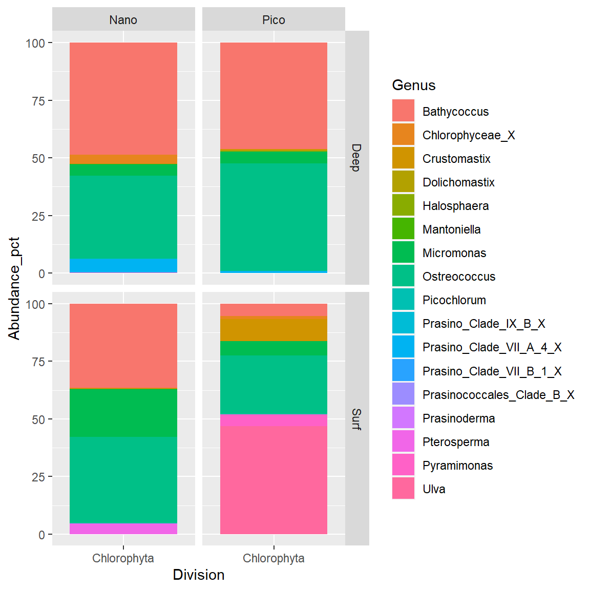

Alpha diversity

Diversity indexes

• Chao1: richness estimator
• Shannon: diversity estimator.

Other include: “Observed”, “ACE”, “Simpson”, “InvSimpson”, “Fisher”

plot_richness(carbom, 
              measures=c("Chao1", "Shannon"))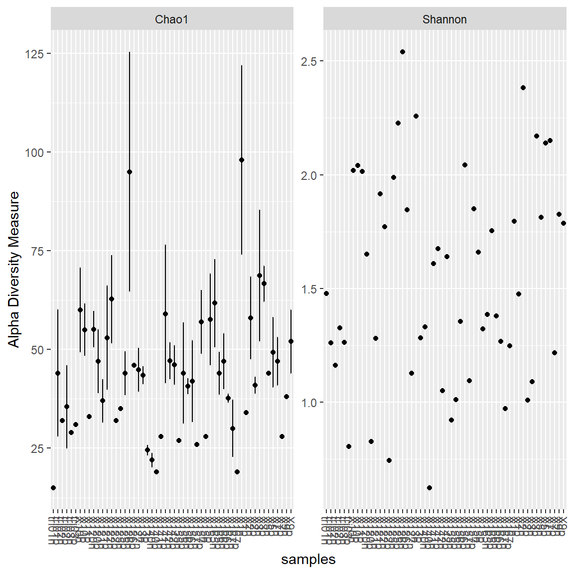

Regroup together samples by level and fraction.

  plot_richness(carbom, measures=c("Chao1", "Shannon"), 
                x="level", 
                color="fraction")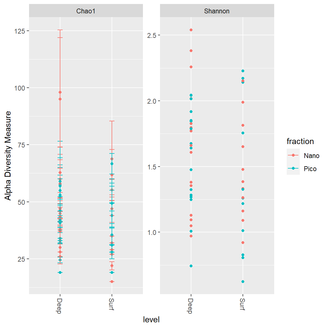

Beta diversity

NMDS

• Ordination: NMDS
• Distance: Bray

carbom.ord <- ordinate(carbom, 
                       method ="NMDS", 
                       distance ="bray")

Square root transformation
Wisconsin double standardization
Run 0 stress 0.2317058 
Run 1 stress 0.2554091 
Run 2 stress 0.2541521 
Run 3 stress 0.244086 
Run 4 stress 0.2467867 
Run 5 stress 0.2515843 
Run 6 stress 0.2458829 
Run 7 stress 0.2588258 
Run 8 stress 0.2399245 
Run 9 stress 0.2526569 
Run 10 stress 0.2460093 
Run 11 stress 0.2508037 
Run 12 stress 0.2618731 
Run 13 stress 0.2412877 
Run 14 stress 0.2482059 
Run 15 stress 0.2294626 
... New best solution
... Procrustes: rmse 0.09894239  max resid 0.3902299 
Run 16 stress 0.2541231 
Run 17 stress 0.2486373 
Run 18 stress 0.2478466 
Run 19 stress 0.2508294 
Run 20 stress 0.2316124 
*** Best solution was not repeated -- monoMDS stopping criteria:
    18: stress ratio > sratmax
     2: scale factor of the gradient < sfgrmin

Plot OTUs

plot_ordination(carbom, 
                carbom.ord, 
                type="taxa", 
                color="Division", 
                title="OTUs")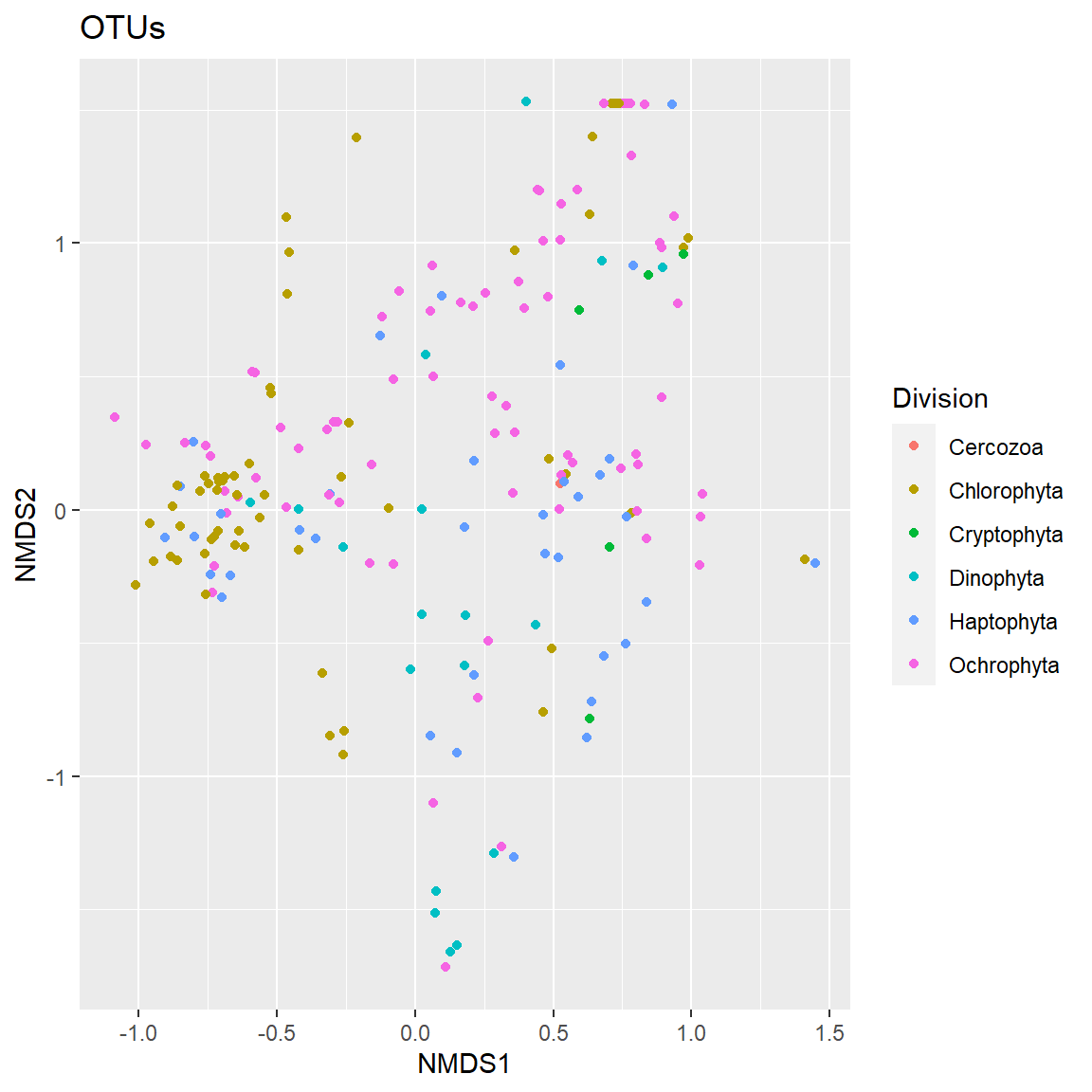

Plot OTUs

A bit confusing, so make it more easy to visualize by breaking according to taxonomic division.

plot_ordination(carbom, 
                carbom.ord, 
                type="taxa", 
                color="Class", 
                title="OTUs", 
                label="Class") +
  facet_wrap(vars(Division), 3)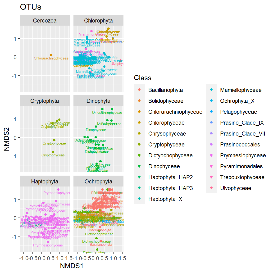

Plot Samples

Enlarge the points to make it more easy to read.

plot_ordination(carbom, 
                carbom.ord, 
                type="samples", 
                color="fraction", 
                shape="level", 
                title="Samples") + 
  geom_point(size=3)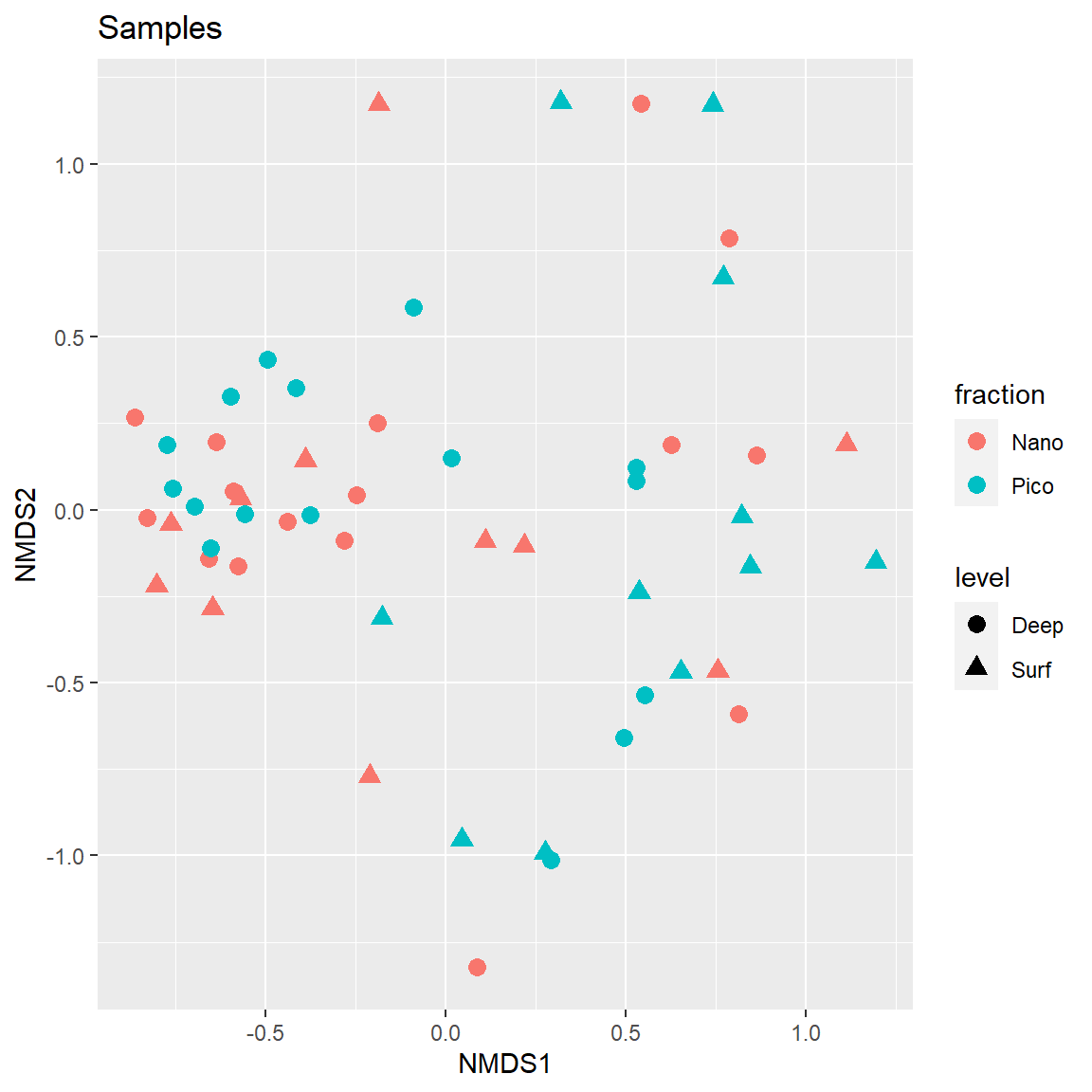

Plot both OTUs and Samples

Two different panels

plot_ordination(carbom, 
                carbom.ord, 
                type="split", 
                color="Division", 
                shape="level", 
                title="biplot", 
                label = "station") +  
  geom_point(size=3)

Methods

CCA - Performs correspondence analysis, or optionally, constrained correspondence analysis (a.k.a. canonical correspondence analysis), via cca

RDA - Performs redundancy analysis, or optionally principal components analysis, via rda

NMDS - Performs Non-metric MultiDimenstional Scaling of a sample-wise ecological distance matrix onto a user-specified number of axes, k. By default, k=2, but this can be modified as a supplementary argument.

MDS/PCoA - Performs principal coordinate analysis (also called principle coordinate decomposition, multidimensional scaling (MDS), or classical scaling) of a distance matrix (Gower 1966), including two correction methods for negative eigenvalues. See pcoa for further details.

Distances

• manhattan
• euclidean
• canberra
• bray
• kulczynski
• jaccard
• gower
• altGower
• morisita
  
• horn
• mountford
• raup
• binomial
• chao
• cao
• unifrac

Heatmaps

Basic heatmap using the default parameters.

  plot_heatmap(carbom, 
               method = "NMDS", 
               distance = "bray")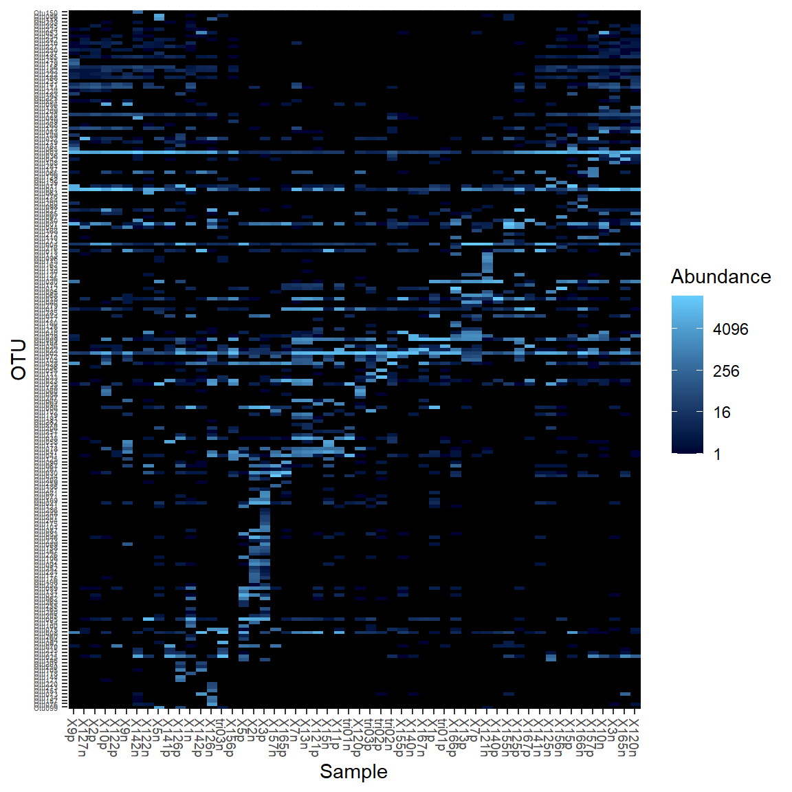

Consider only main OTUS

It is very very cluttered. It is better to only consider the most abundant OTUs for heatmaps. For example one can only take OTUs that represent at least 20% of reads in at least one sample. Remember we normalized all the sampples to median number of reads (total). We are left with only 33 OTUS which makes the reading much more easy.

  carbom_abund <- filter_taxa(carbom, 
                              function(x) sum(x > total*0.20) > 0, 
                              TRUE)
  carbom_abund

phyloseq-class experiment-level object
otu_table()   OTU Table:         [ 33 taxa and 54 samples ]
sample_data() Sample Data:       [ 54 samples by 27 sample variables ]
tax_table()   Taxonomy Table:    [ 33 taxa by 7 taxonomic ranks ]

  otu_table(carbom_abund)[1:8, 1:5]

OTU Table:          [8 taxa and 5 samples]
                     taxa are rows
        X10n  X10p  X11p X120n X120p
Otu001 13339  7346  3804 12662     3
Otu002    18  8329 14958    30 36206
Otu003  9692 10488    20 16537    11
Otu004  3584  4943    33     7     9
Otu005     0     6    11     0     5
Otu006     0     9     0     0     5
Otu007  4473   605   587  5894     3
Otu008     1     9  6707     2    17

Consider only main OTUS

   plot_heatmap(carbom_abund, 
                method = "NMDS", 
                distance = "bray")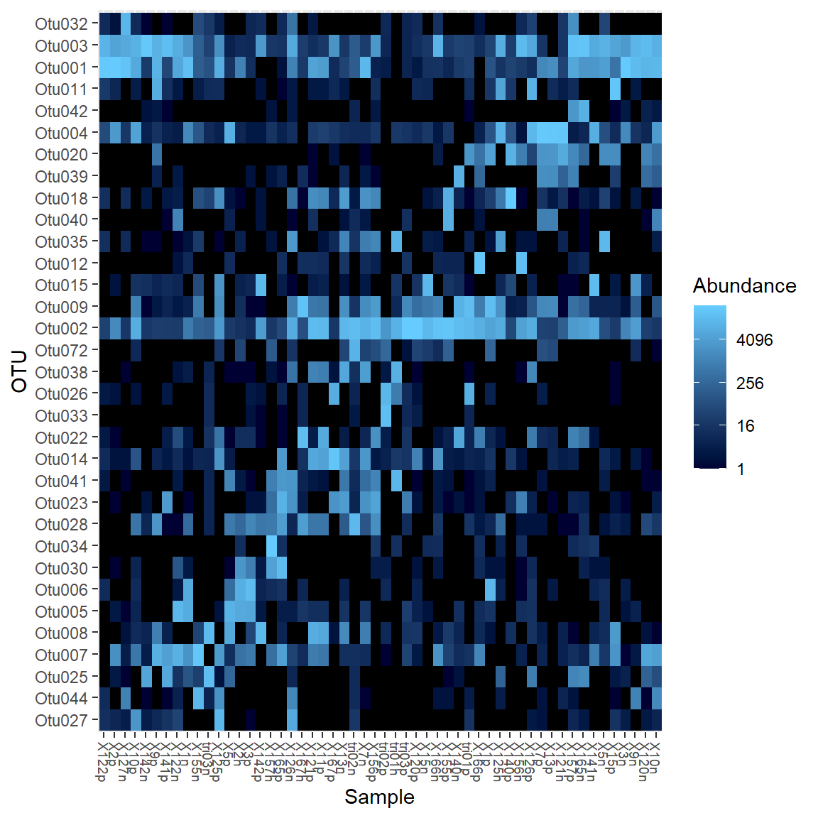

Change distances

It is possible to use different distances and different multivaraite methods. For example Jaccard distance and MDS and label OTUs with Class, order by Class. We can also change the Palette (the default palette is a bit ugly…).

  plot_heatmap(carbom_abund, 
               method = "MDS", 
               distance = "(A+B-2*J)/(A+B-J)", 
               taxa.label = "Class", 
               taxa.order = "Class", 
               trans=NULL, 
               low="beige", 
               high="red", 
               na.value="beige")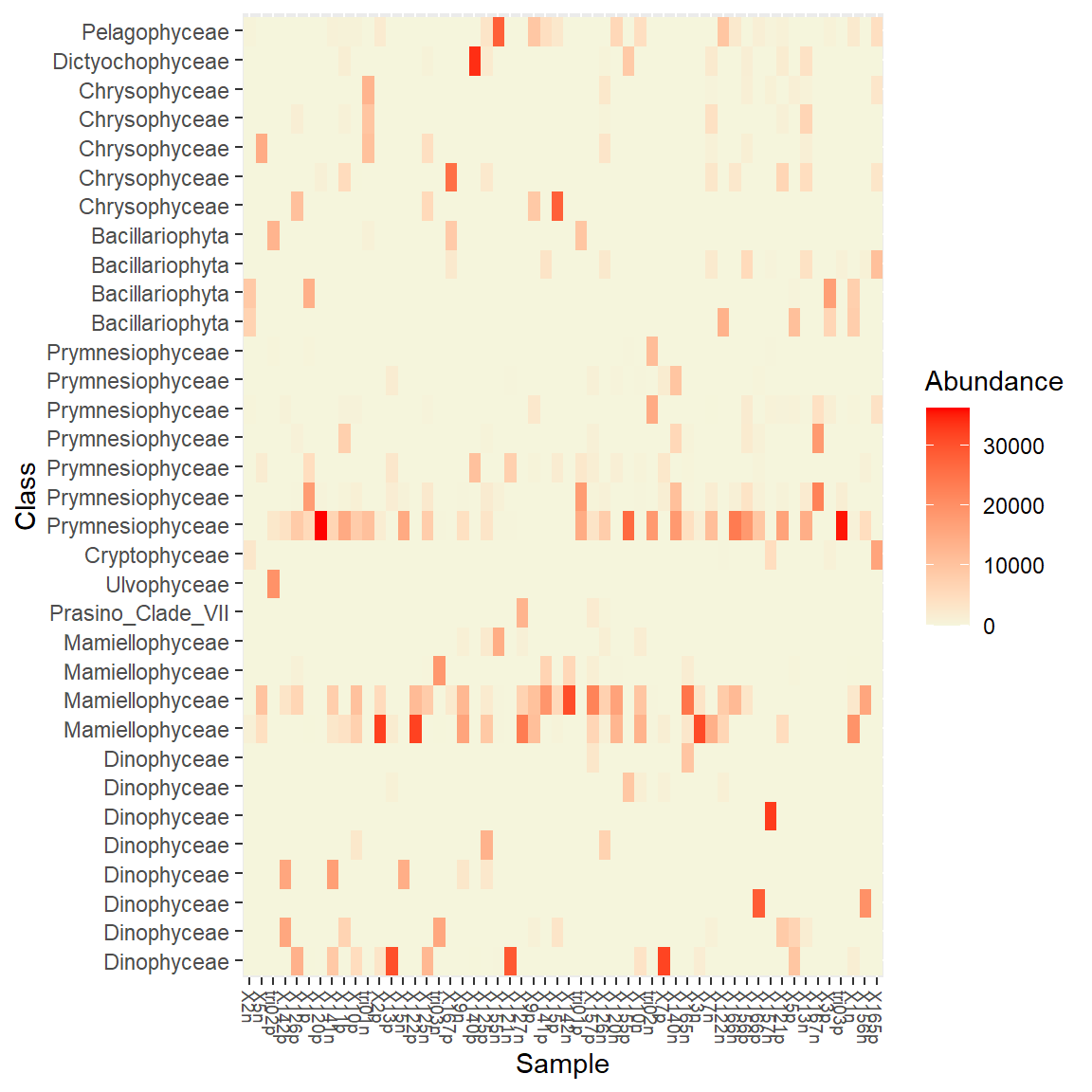

Heatmap for a specific taxonomy group.

For example we can taget the Chlorophyta and then label the OTUs using the Genus.

  plot_heatmap(carbom_chloro_ps, 
               method = "NMDS", 
               distance = "bray", 
               taxa.label = "Genus", 
               taxa.order = "Genus", 
               low="beige", 
               high="red", 
               na.value="beige")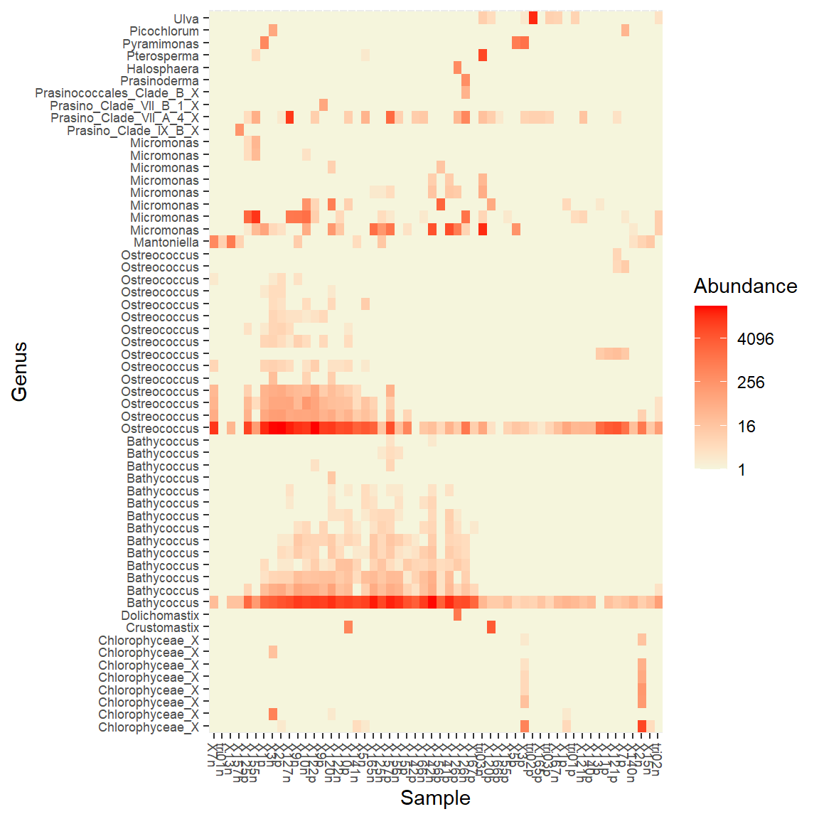

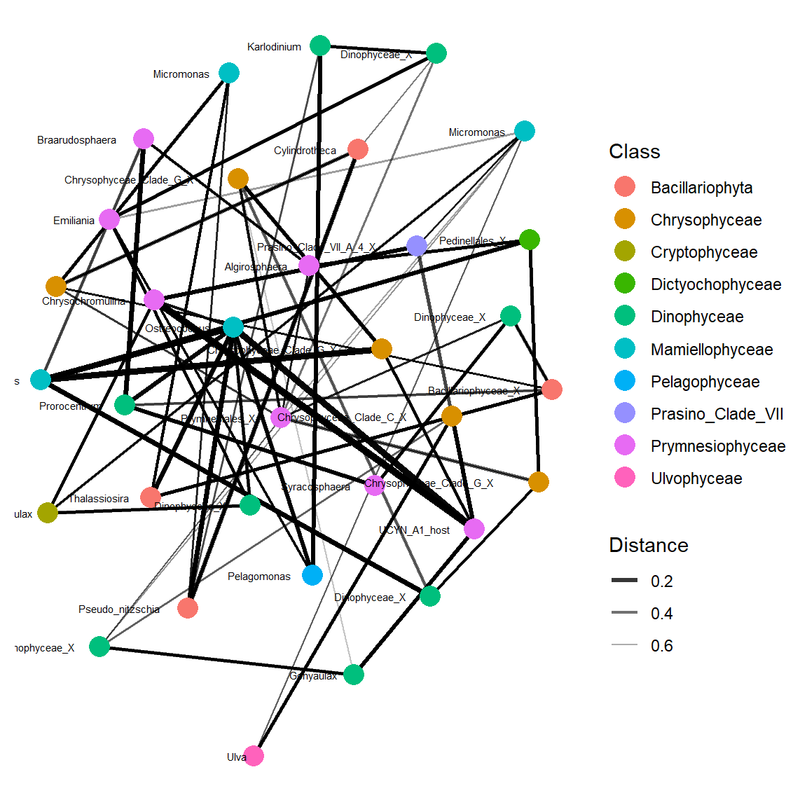
Networks

Simple network analysis

  plot_net(carbom, 
           distance = "(A+B-2*J)/(A+B)", 
           type = "taxa", 
           maxdist = 0.7, 
           color="Class", 
           point_label="Genus")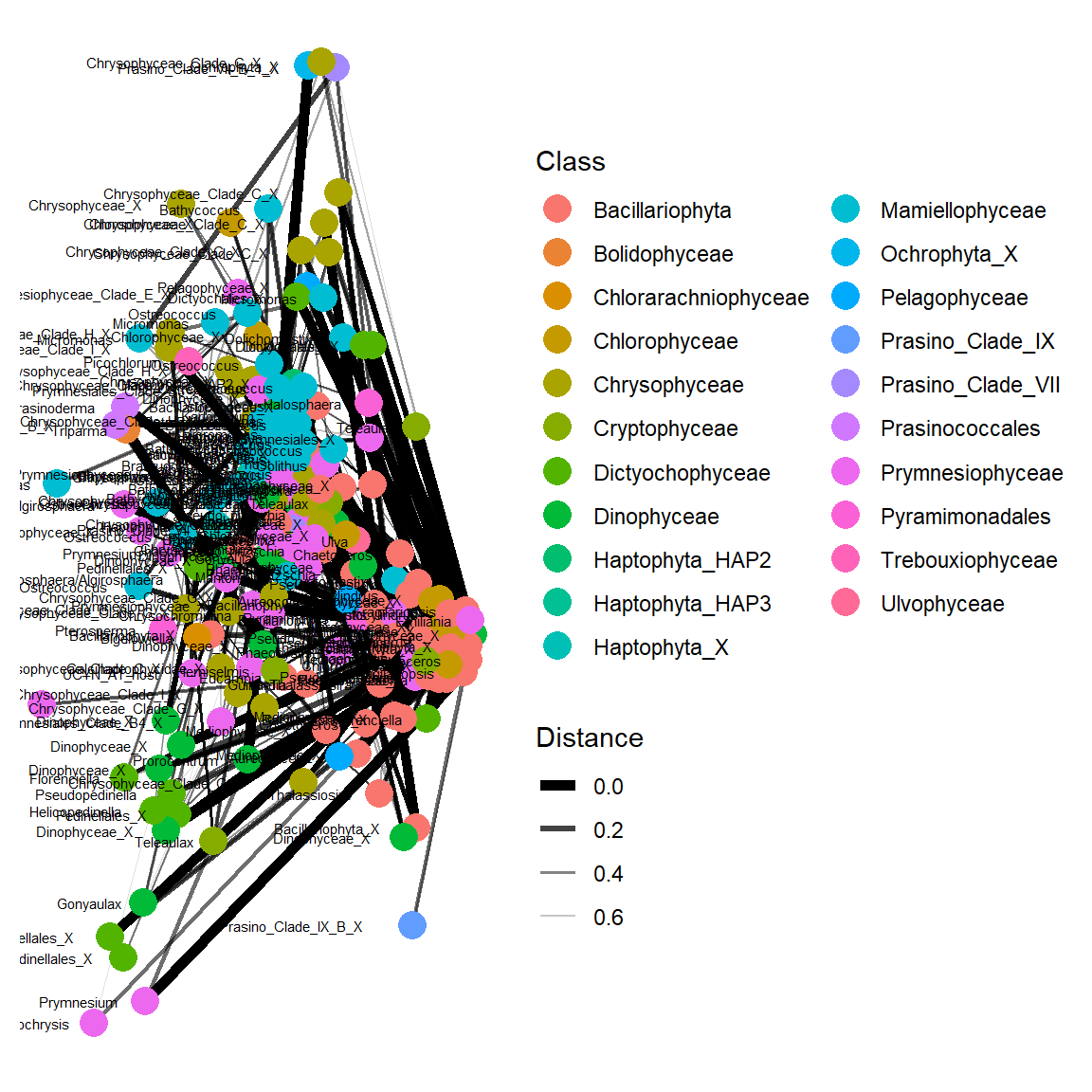

Simplify

Let us make it more simple by using only major OTUs

  plot_net(carbom_abund, 
           distance = "(A+B-2*J)/(A+B)", 
           type = "taxa", 
           maxdist = 0.8, 
           color="Class", 
           point_label="Genus") 

What did we learn ?

• Create file
• Bar graphs
• Alpha diversity
• Beta diversity