R course
Daniel Vaulot
2023-01-21
![]()
![]()
![]()
![]()
Data visualization
Installation and Resources
Packages
- ggplot2
- patchwork
Download
- R-session-03.zip
Reading
Resources
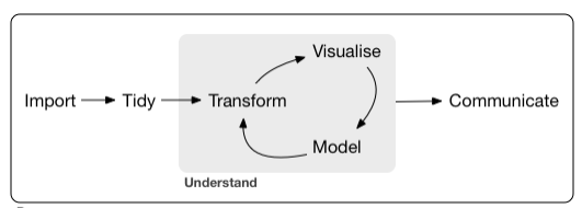
Workflow
Graph purposes
- Analysis graphs
- design to see patterns, trends
- aid the process of data description
- interpretation
- Presentation graphs
- design to attract attention
- make a point
- illustrate a conclusion
Source: Michael Friendly
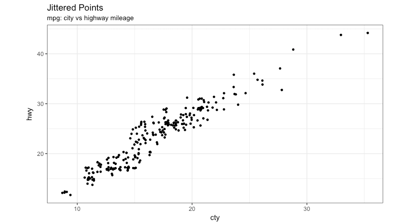
Jitter
- Two variables numerical
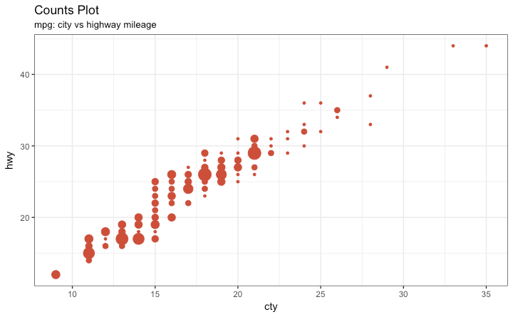
Bubble
- Two variables numerical
- Add another variable numerical
Animate
- Two variables numerical
- One variable numerical
- One variable categorical
- Animate another variable
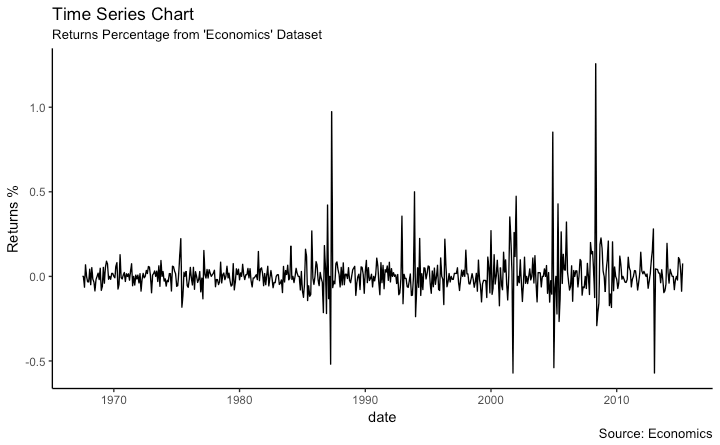
Times series
- Line graph
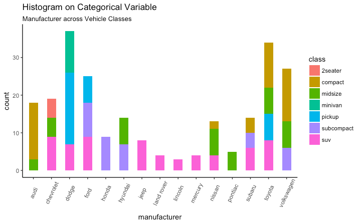
Bargraphs
- One variable categorical
- One variable numerical
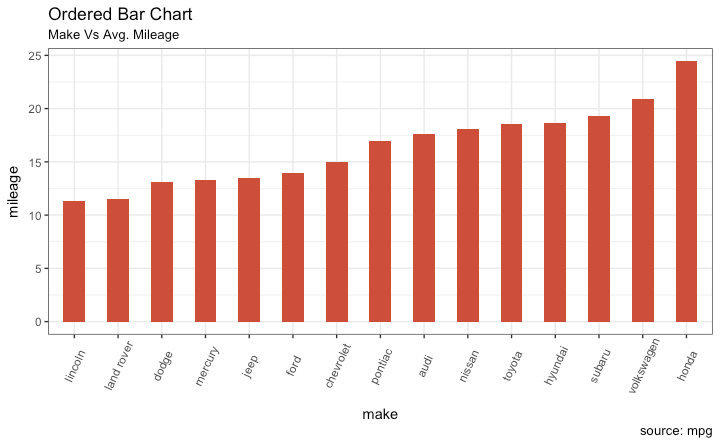
Bargraphs
- Rotate
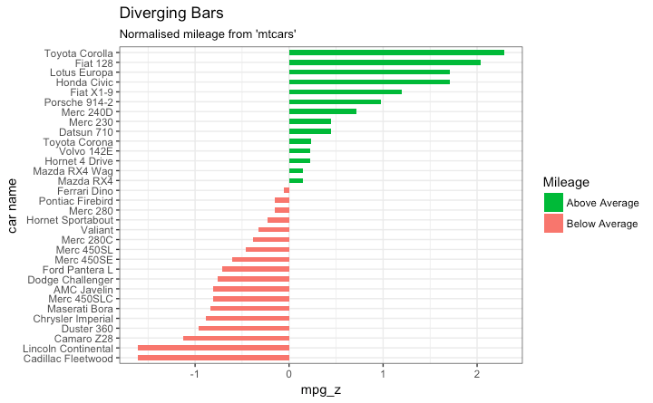
Bargraphs
- Two variable categorical
- One variable numerical
Boxplots
- One variable categorical
- One variable numerical but with many values

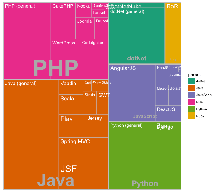
Treemaps
- One variable categorical
- One variable numerical
- Much better than pie charts
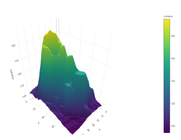
3D
- Three variable numerical
- Avoid unless it is a simple shape
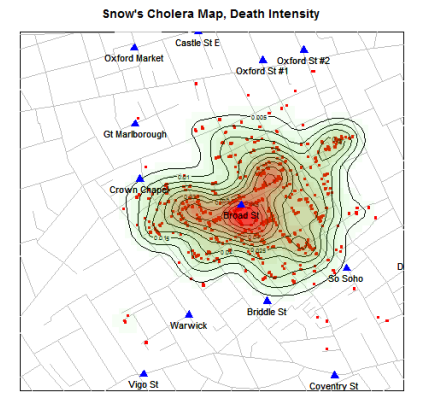
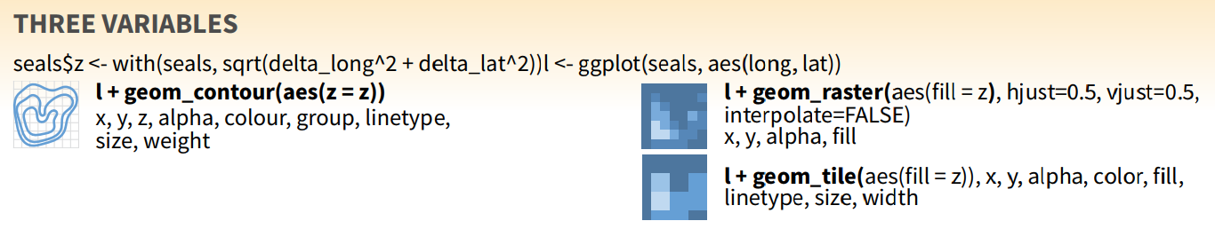
Contours
- Three variable numerical
- Better than 3D
Many…
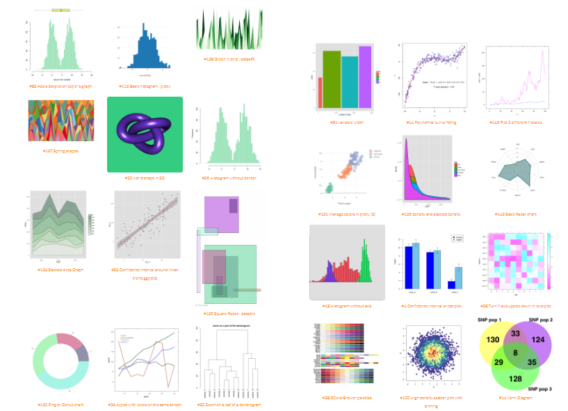
- Choose as a function of what you want to analyze or the story you want to tell
- https://www.r-graph-gallery.com/all-graphs/
@allison_horst
A simple plot
- Choose the data set
- Choose the geometric representation
- Choose the aesthetics : x,y, color, shape etc…
# All functions are from ggplot2 package unless specified

ggplot(data=samples) +
    geom_point(mapping = aes(x=phosphates,
                            y=nitrates))
The grammar of graphics

 ggplot(data=samples) +
  geom_point(mapping = aes(x=phosphates,
                           y=nitrates))
Every graph can be described as a combination of independent building blocks:
- data: a data frame: quantitative, categorical; local or data base query
- aesthetic mapping of variables into visual properties: size, color, x, y
- geometric objects (“geom”): points, lines, areas, arrows, …
- coordinate system (“coord”): Cartesian, log, polar, map
Alternatively
- Move mapping into ggplot function
 ggplot(data=samples,
        mapping = aes(x=phosphates,
                      y=nitrates)) +
  geom_point()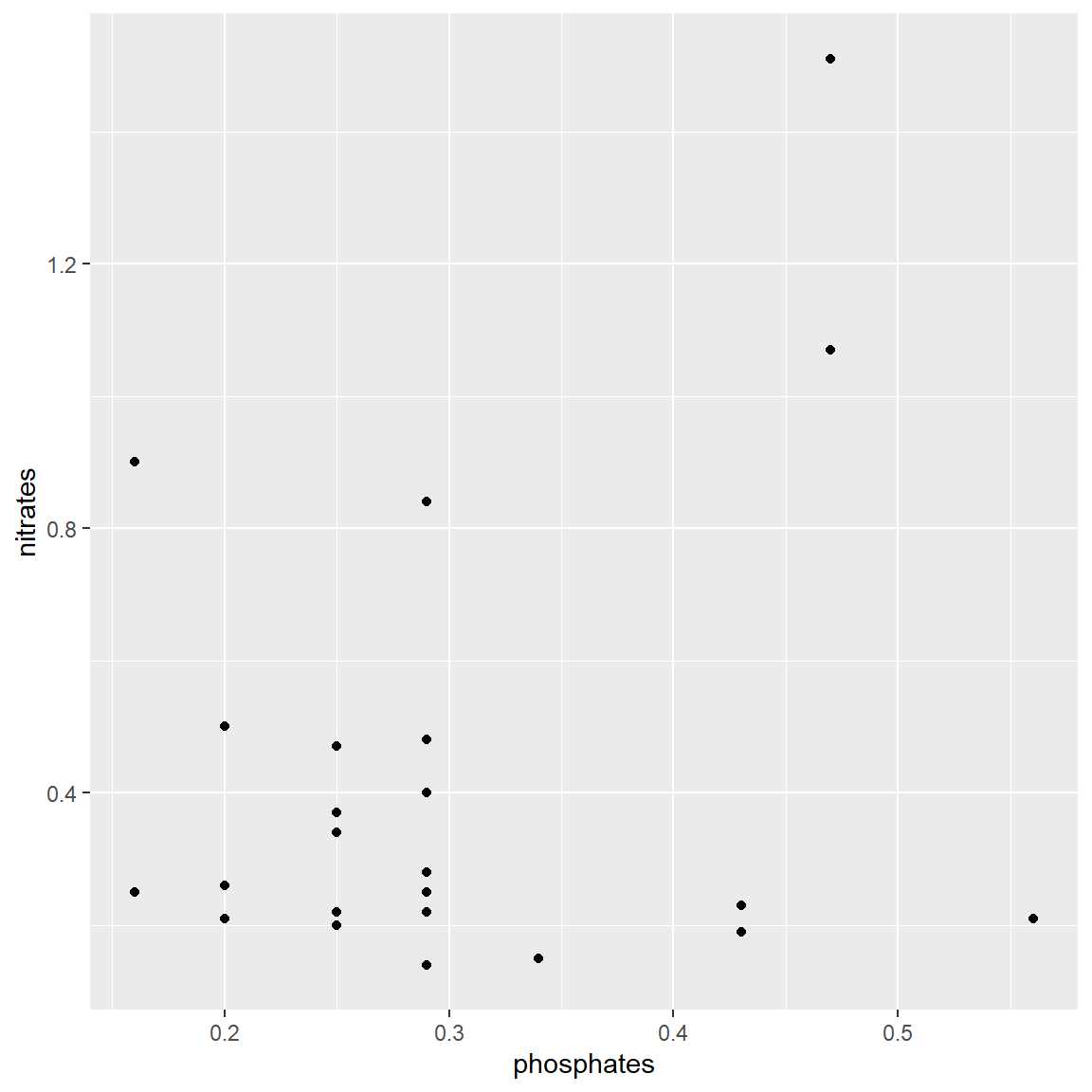
Alternatively
- Remove function arguments
 ggplot(samples,
        aes(x=phosphates,
            y=nitrates)) +
  geom_point()
Makes dots bigger
- Add: size=5 outside of the aesthetics function
 ggplot(samples,
        aes(x=phosphates,
            y=nitrates)) +
  geom_point(size=5)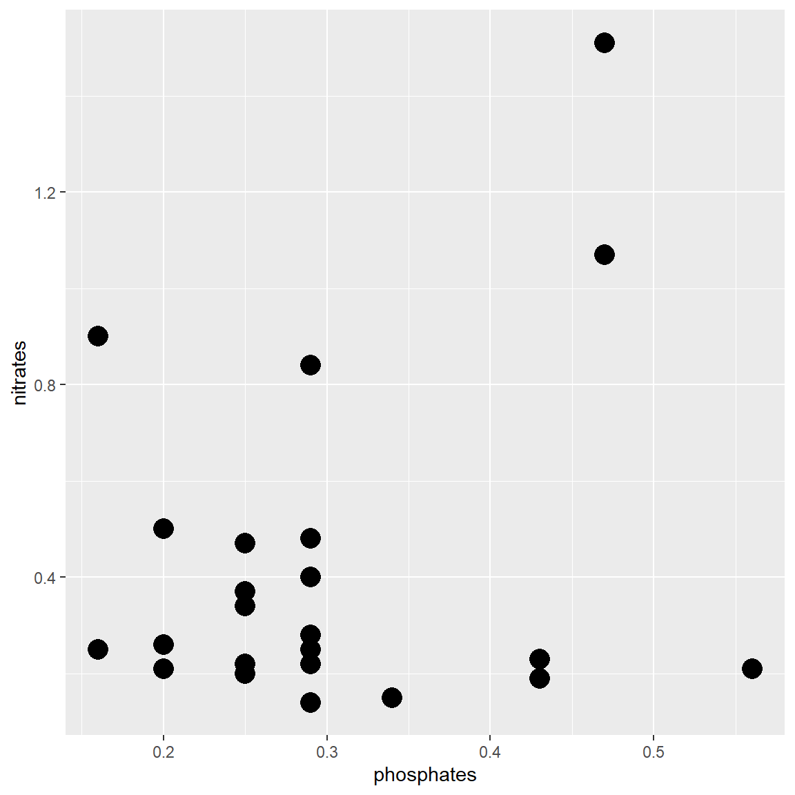
Color according to depth level (discrete)
- The mapping aesthetics must be an argument of the aes function
- geom_point(color=level, size=5) will generate an error…
 ggplot(samples,
        aes(x=phosphates,
            y=nitrates,
            color=level)) +
  geom_point(size=5)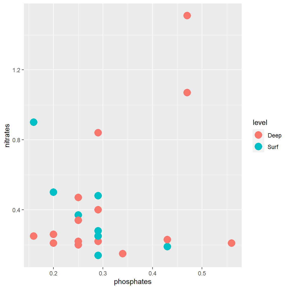
Color according to depth (continuous)
- The mapping aesthetics must be an argument of the aes function
- Add: color=depth
 ggplot(samples,
        aes(x=phosphates,
            y=nitrates,
            color=depth)) +
  geom_point(size=5)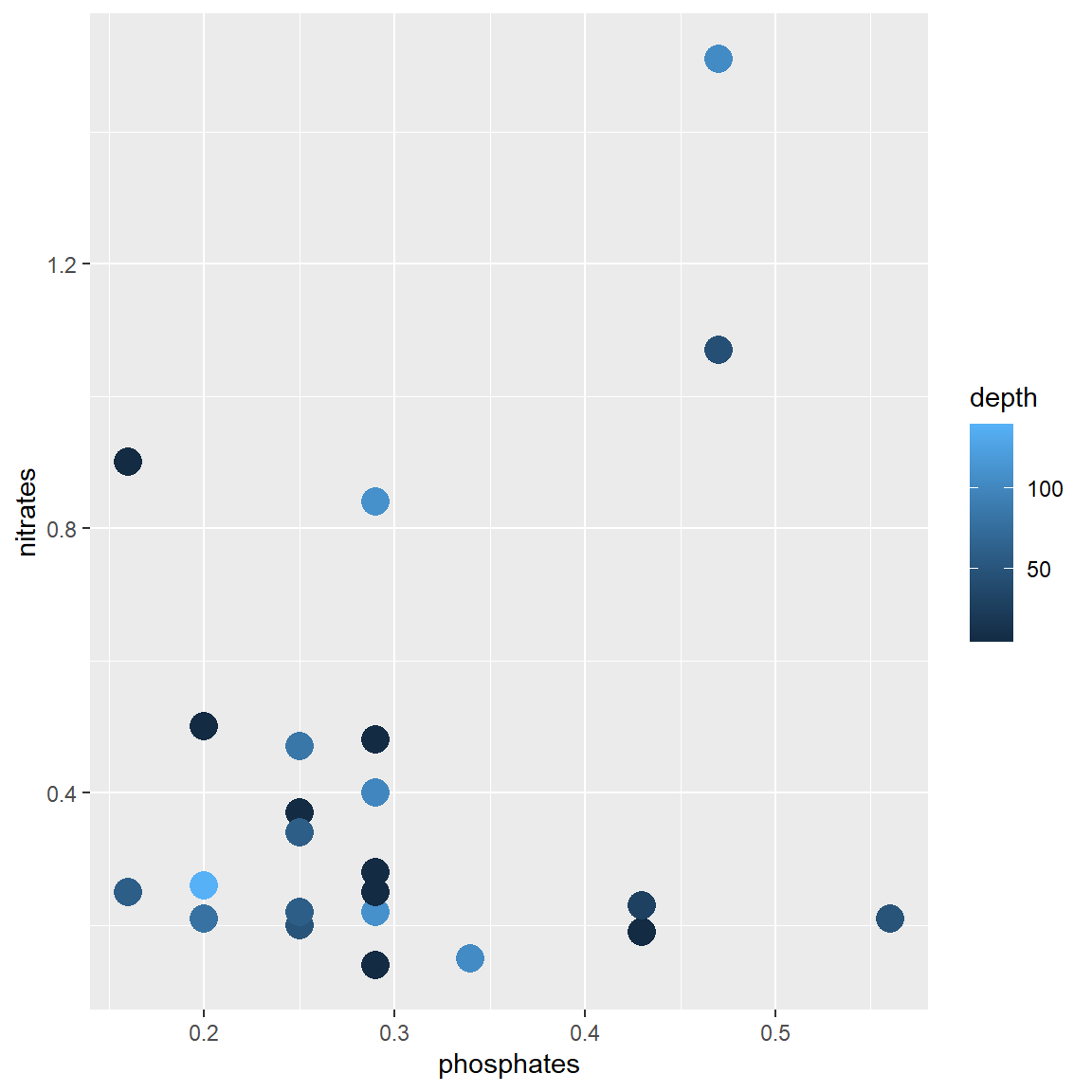
Symbol according to transect (continuous)
- Add: shape=as.character(transect)
 ggplot(samples,
        aes(x=phosphates,
            y=nitrates,
            color=depth,
            shape=as.character(transect))) +
  geom_point(size=5)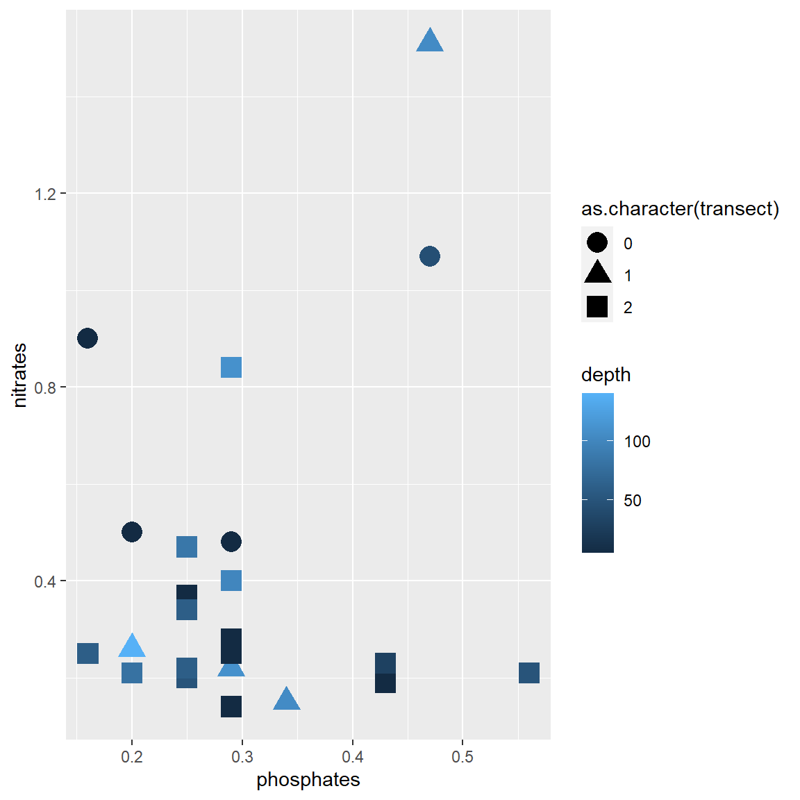
Panels depending on one variable
 ggplot(samples,
        aes(x=phosphates,
            y=nitrates)) +
  geom_point() +
facet_wrap(~ level) 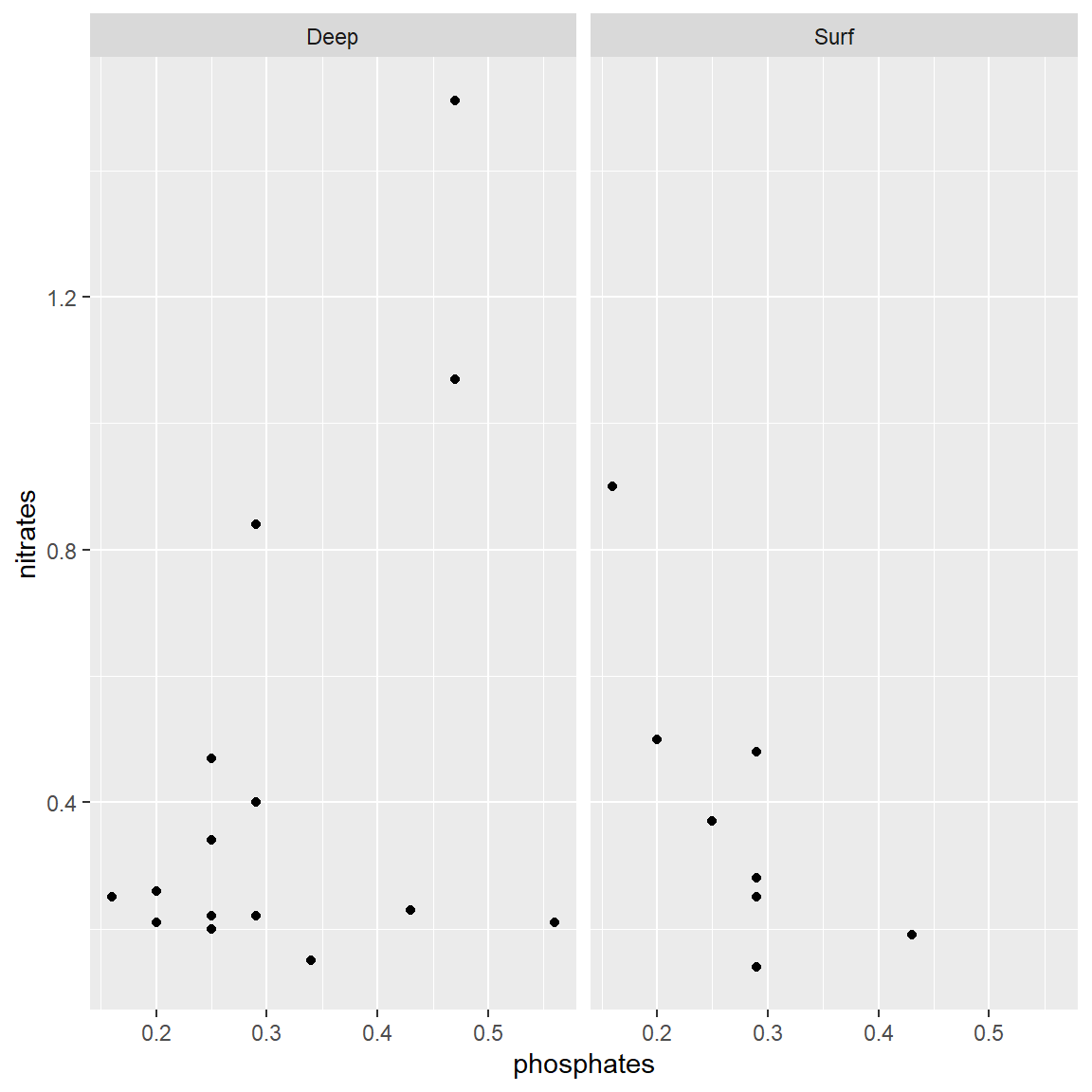
Adding a regression line
- Add: geom_smooth()
- You can choose the type of smoothing “lm” is for linear model
 ggplot(samples,
        aes(x=phosphates,
            y=nitrates,
            color=level)) +
  geom_point(size=5) +
  geom_smooth(mapping = aes(x=phosphates,
                            y=nitrates),
              method="lm")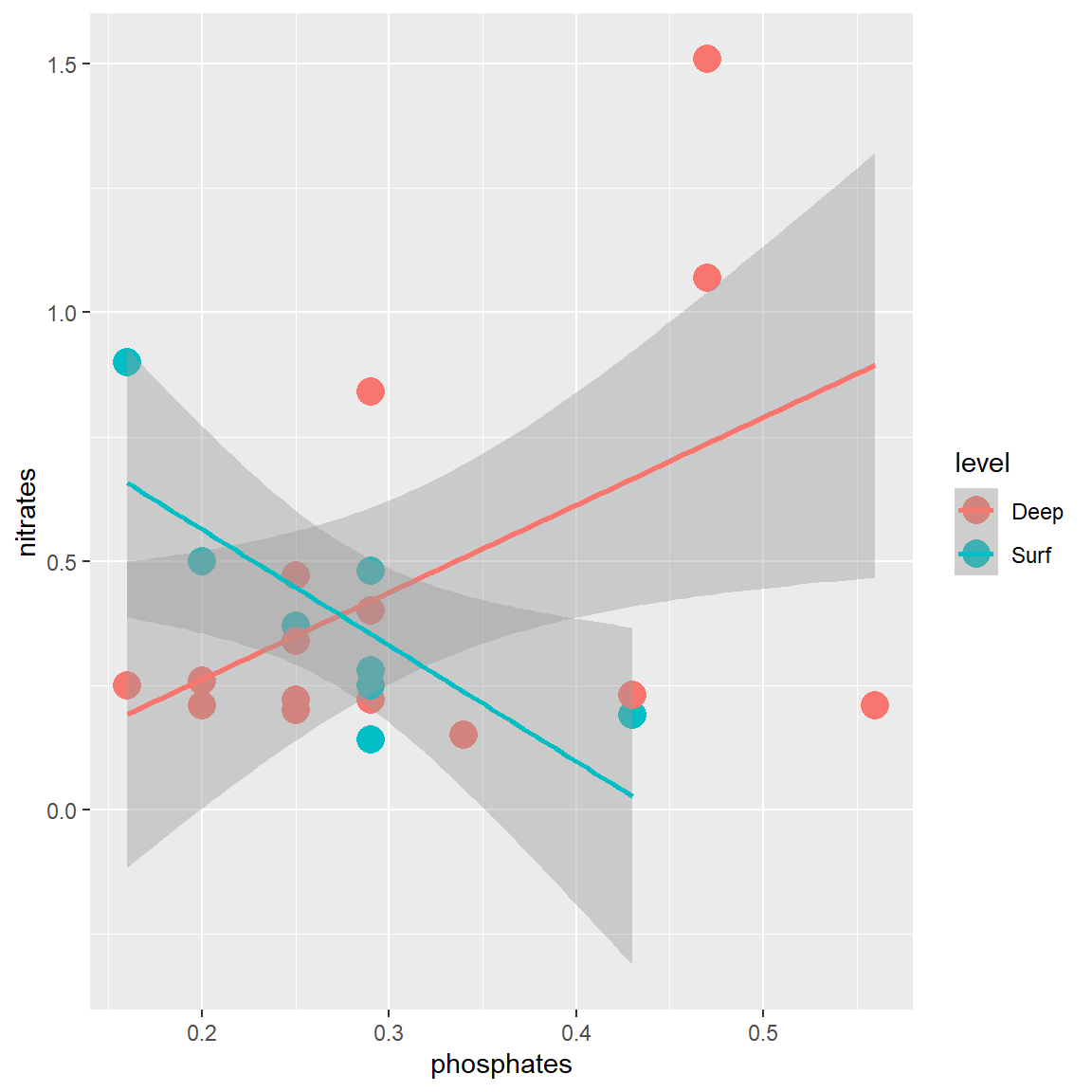
Adding a regression line
- If the mapping is in the ggplot function is for all the geom….
 ggplot(samples,
        aes(x=phosphates,
            y=nitrates)) +
  geom_point(aes(color=level),
             size=5) +
  geom_smooth(mapping = aes(x=phosphates,
                            y=nitrates),
              method="lm")
Finalizing the graph
- Adding labels and legends
 ggplot(samples) +
  geom_point(mapping = aes(x=phosphates,
                           y=nitrates,
                           color=level),
             size=5) +
  geom_smooth(mapping = aes(x=phosphates,
                            y=nitrates),
              method="lm") +
  xlab("Phosphates") +
  ylab("Nitrates") +
  ggtitle("CARBOM cruise")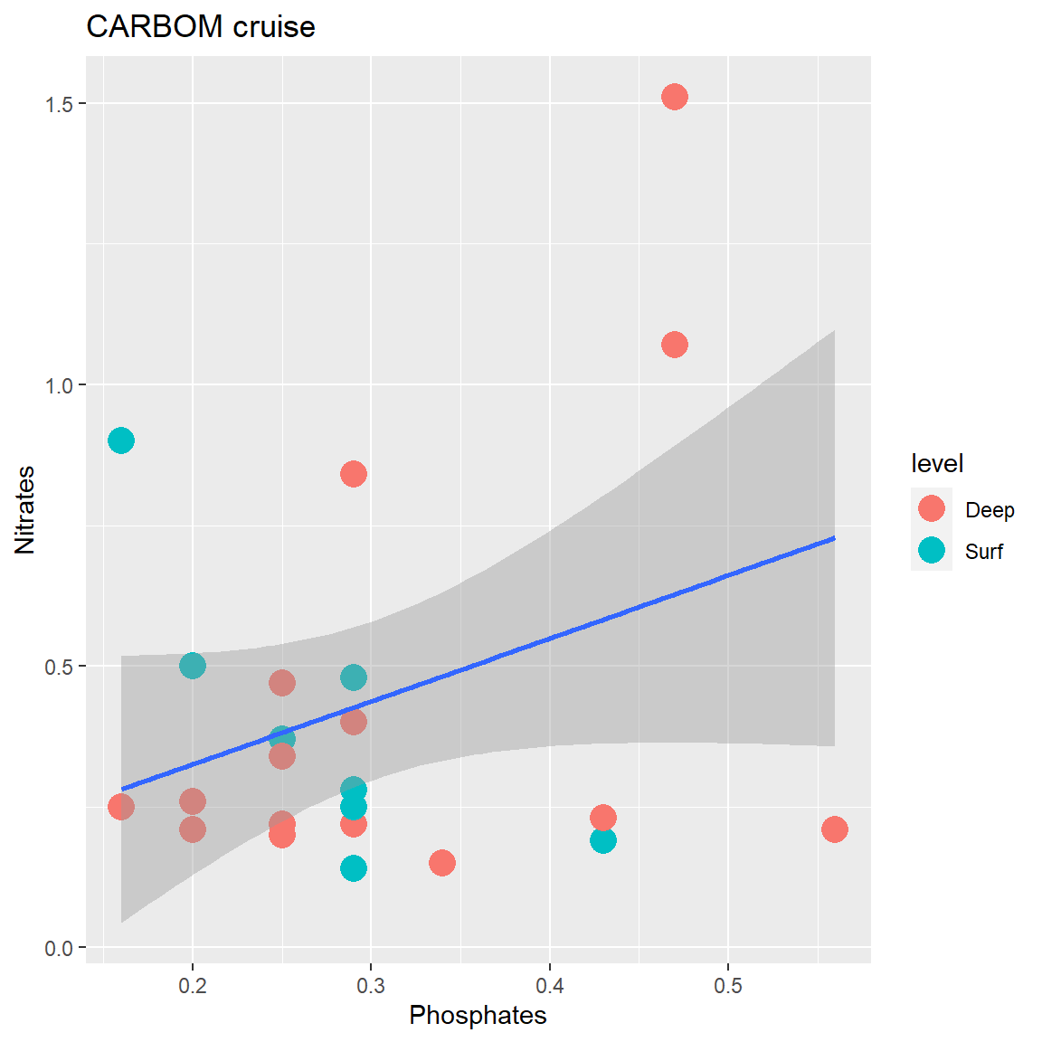
First graph
 g1 <- ggplot(samples) +
  geom_point(mapping = aes(x=phosphates,
                           y=nitrates,color=
                             level), size=5) +
  geom_smooth(mapping = aes(x=phosphates,
                            y=nitrates),
              method="lm") +
  xlab("Phosphates") +
  ylab("Nitrates")

 g1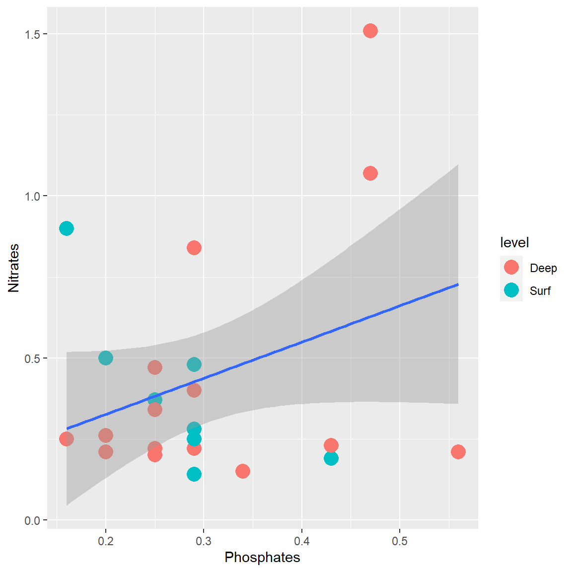
Second graph
 g2<- ggplot(samples) +
  geom_point(mapping = aes(x=nanoeuks,
                           y=picoeuks,
                           color=level),
             size=5) +
  geom_smooth(mapping = aes(nanoeuks,
                            y=picoeuks),
              method="lm") +
  xlab("Pico-eukaryotes") +
  ylab("Nano-eukaryotes")

 g2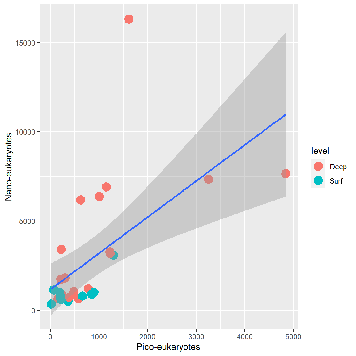
Package patchwork
- https://patchwork.data-imaginist.com/index.html
- See also packages :
gridExtracowplot
library(patchwork)
(g1 / g2)
Package patchwork
- Adding annotation
- Collecting legends
g1 / g2 +
  plot_annotation(tag_levels = 'A') +
  plot_layout(guides = 'collect')
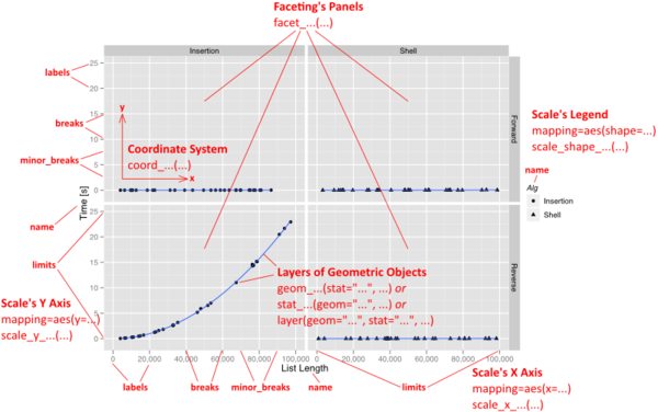
Anatomy of a plot
Geometries

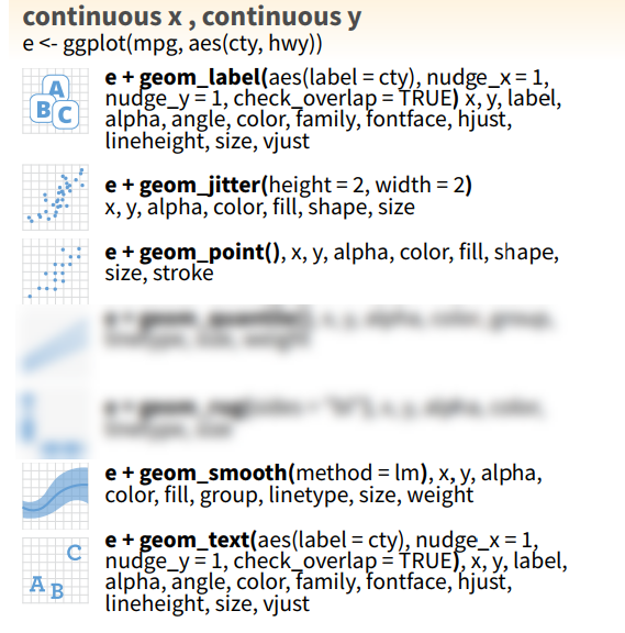
Continuous x and y
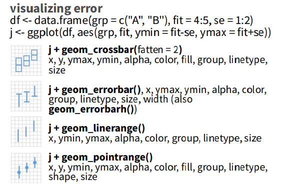
Plotting error
Discrete x - Continuous y

Continuous x

3D
Modifying axis and scales

Palettes
- Package tmaptools : https://github.com/mtennekes/tmaptools
- Function :
palette_explorer()
- Function :
- Package paletteer : https://github.com/EmilHvitfeldt/paletteer
- More than 1000 palettes
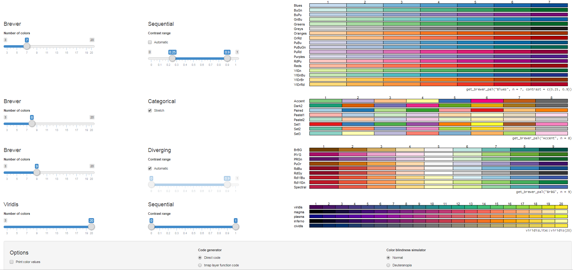
Palettes
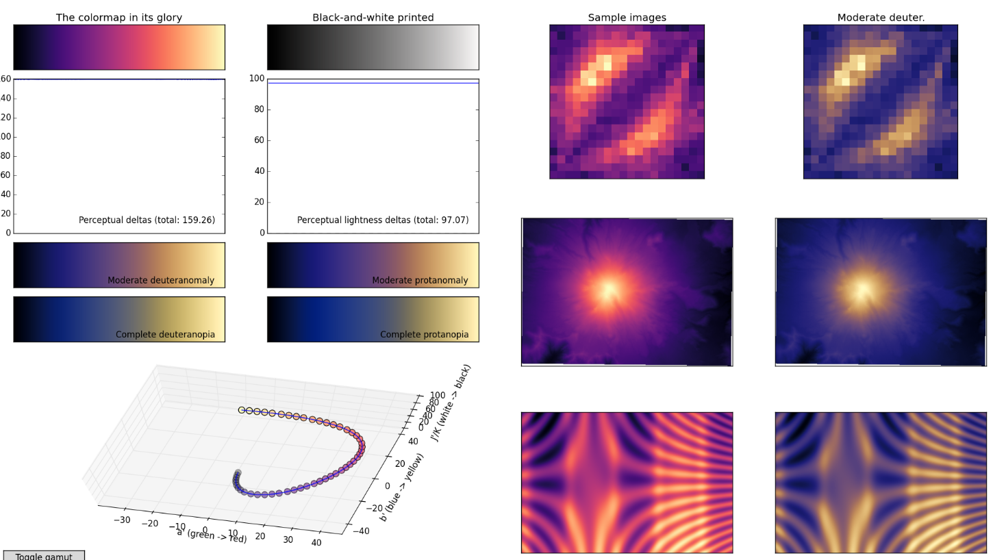
- Use color blind friendly palettes
- viridis (e.g.
scale_colour_viridis_c())
- viridis (e.g.
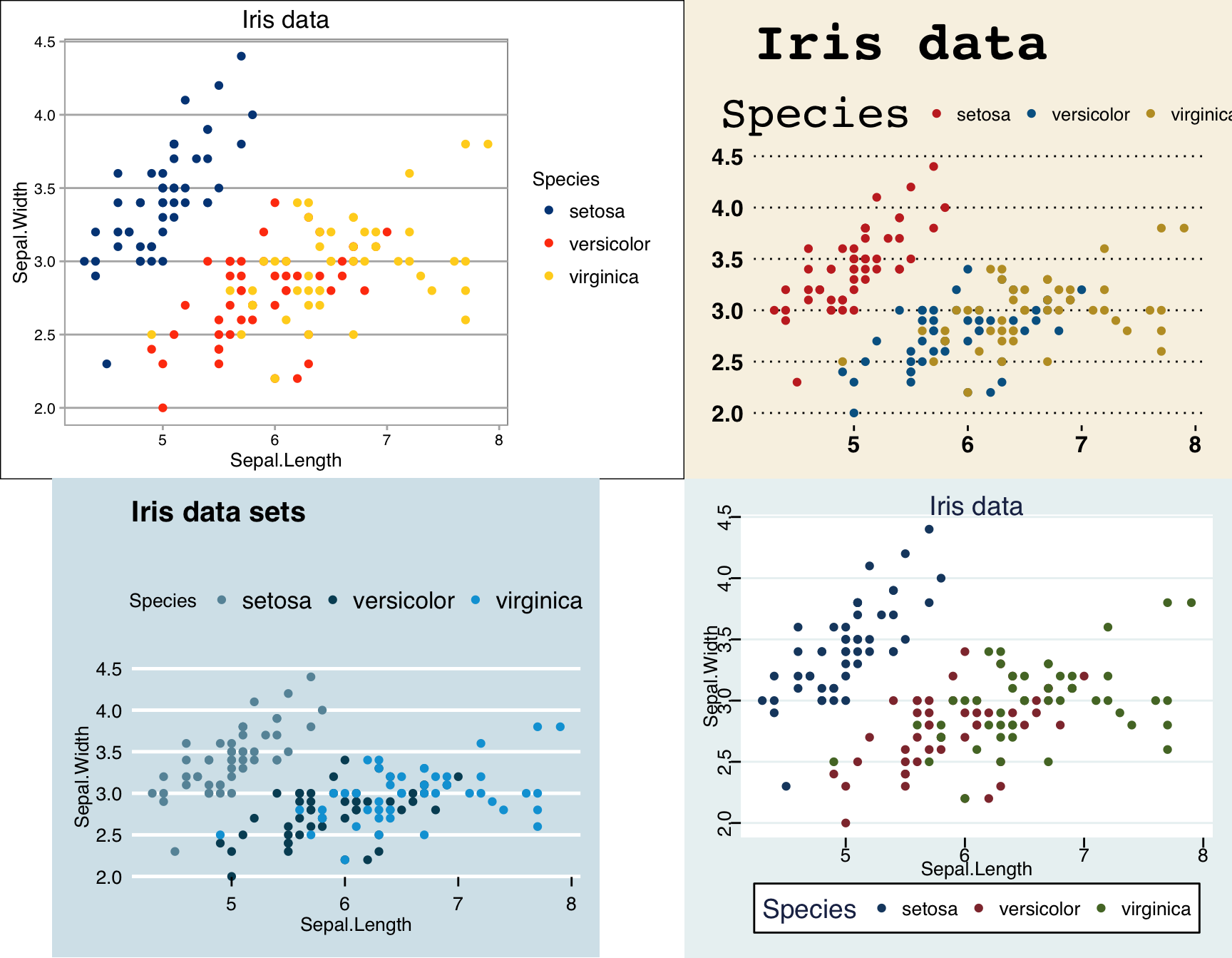
Themes
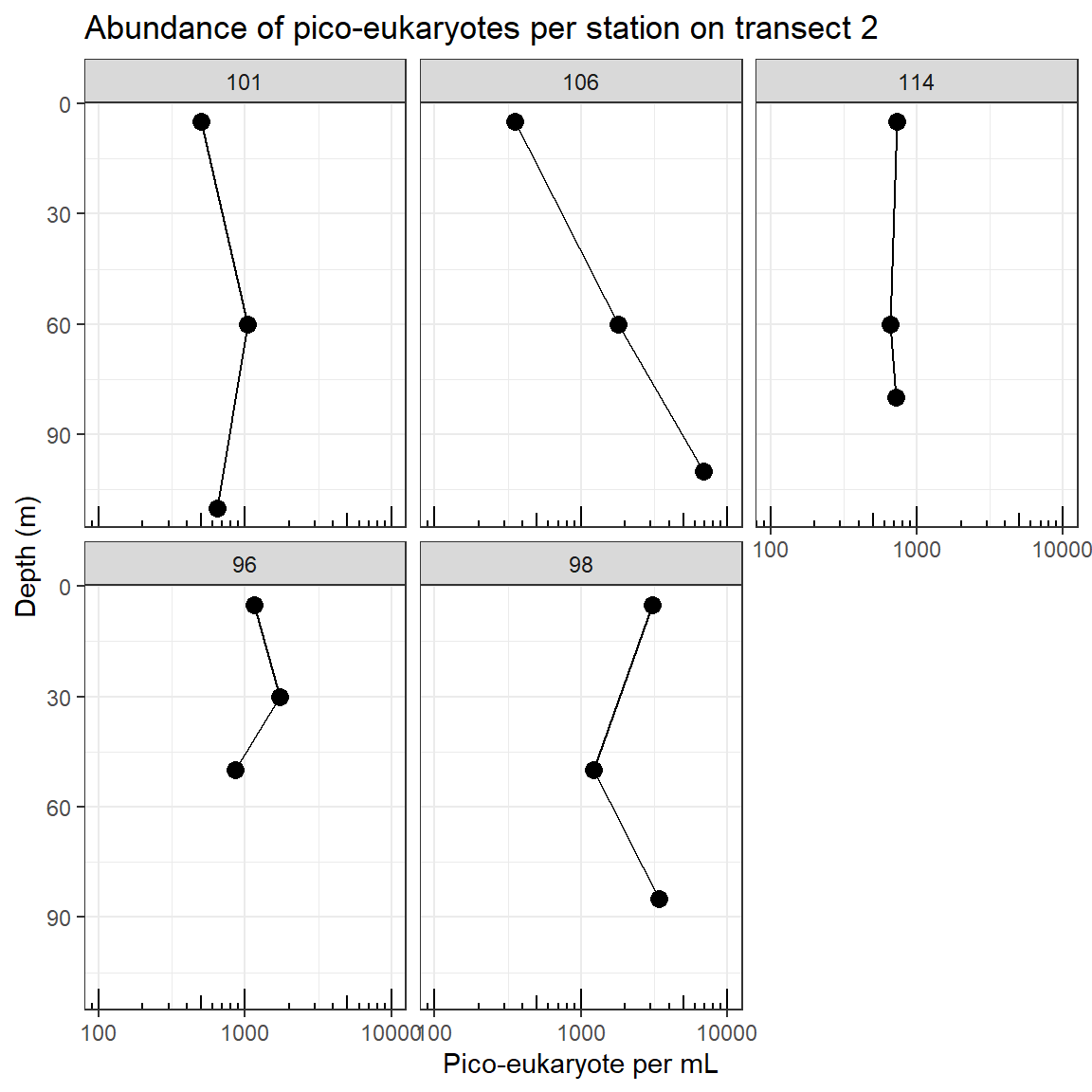
Your mission
Reproduce graph on right
- Only transect 2
- One panel per station
- Increasing depth
- Log scale for x
- White background
Instructions
- Work by group of 2 (1 expert, 1 less expert)
- Send code and results by element.io

Step 1
- basic plot
ggplot(filter(samples,
               transect==2 & !is.na(depth)),
        aes(y=depth, x=picoeuks))  +
geom_point(size=3)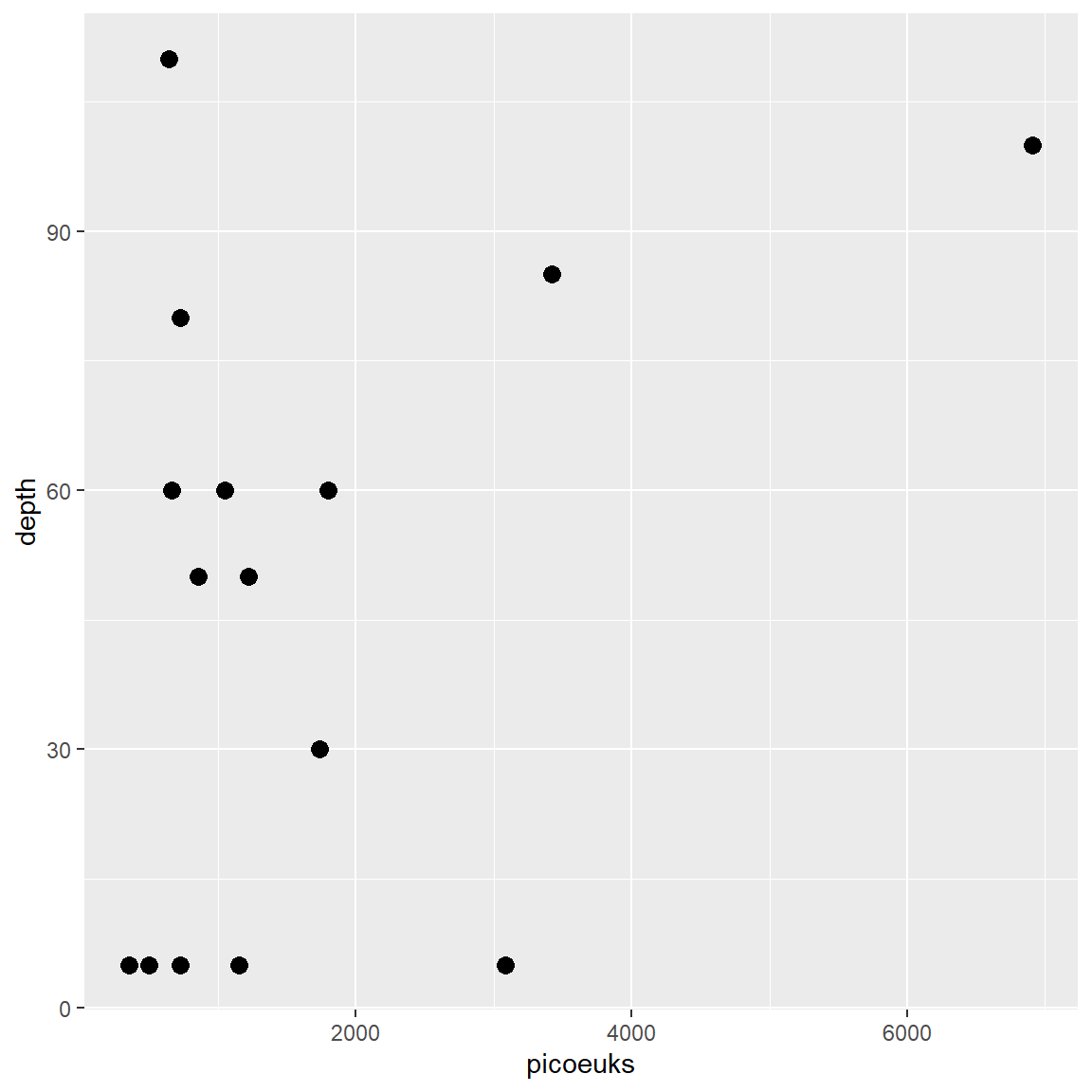
Step 2
- facet_wrap
ggplot(filter(samples,
             transect==2 & !is.na(depth)),
      aes(y=depth, x=picoeuks))  +
geom_point(size=3) +
facet_wrap(~ station) 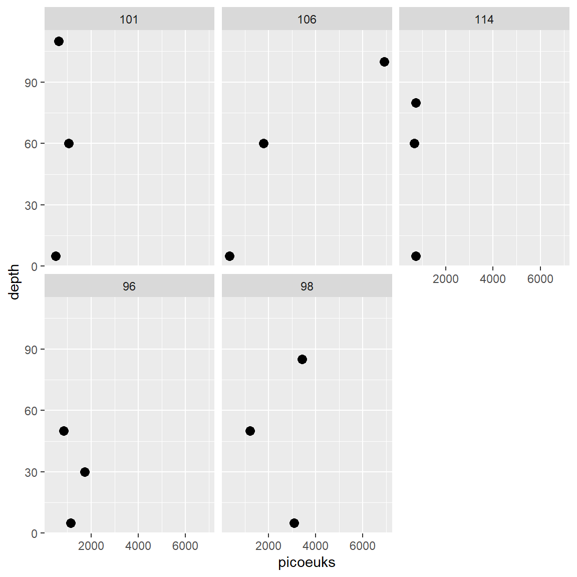
Step 3
- link points together (! use geom_path())
ggplot(filter(samples,
             transect==2 & !is.na(depth)),
      aes(y=depth, x=picoeuks))  +
geom_point(size=3) +
facet_wrap(~ station) +
geom_path() 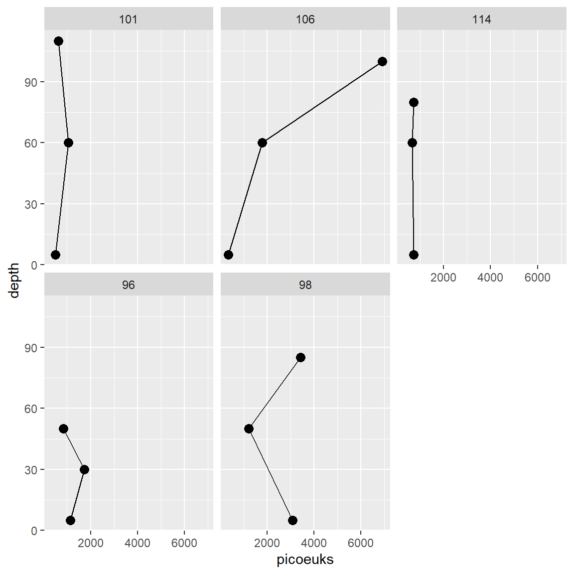
Step 4
- reverse y scale
ggplot(filter(samples,
             transect==2 & !is.na(depth)),
      aes(y=depth, x=picoeuks))  +
geom_point(size=3) +
facet_wrap(~ station) +
geom_path() +
scale_y_reverse() 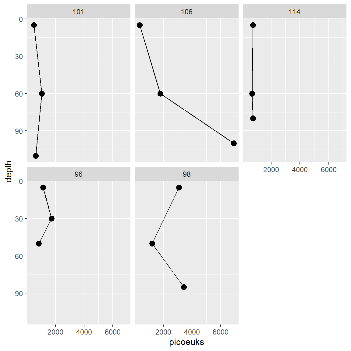
Step 5
- add theme
ggplot(filter(samples,
             transect==2 & !is.na(depth)),
      aes(y=depth, x=picoeuks))  +
geom_point(size=3) +
facet_wrap(~ station) +
geom_path() +
scale_y_reverse() +
theme_bw()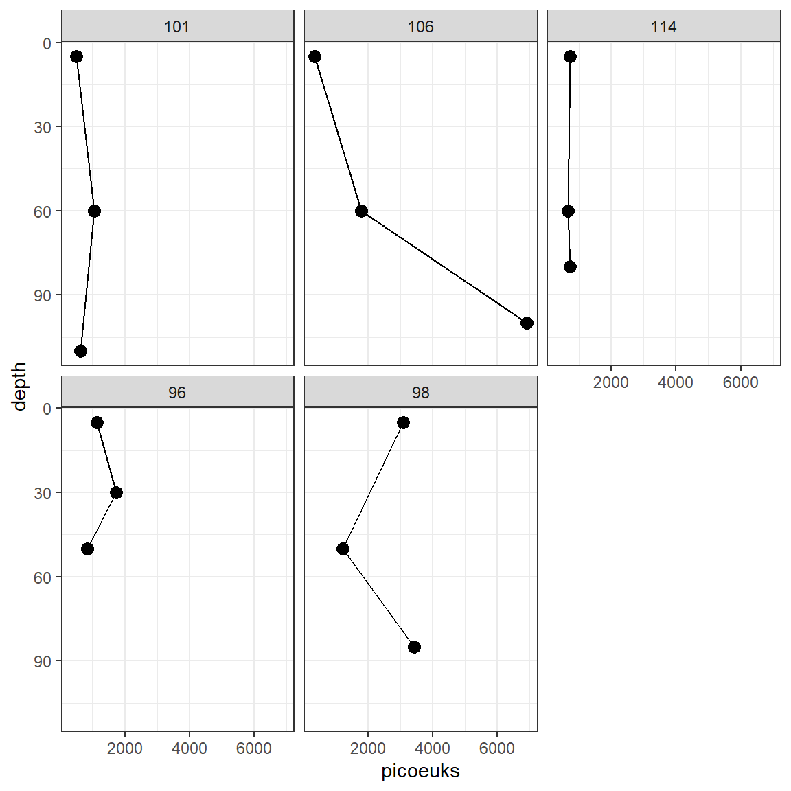
Step 6
- add legends
ggplot(filter(samples,
             transect==2 & !is.na(depth)),
      aes(y=depth, x=picoeuks))  +
geom_point(size=3) +
facet_wrap(~ station) +
geom_path() +
scale_y_reverse() +
theme_bw() +
ggtitle("Abundance of pico-eukaryotes per station on transect 2") +
xlab("Pico-eukaryote per mL") +
ylab("Depth (m)") 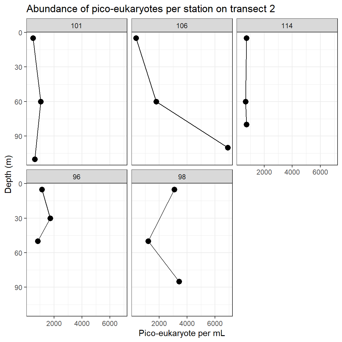
Step 7
- change scales
ggplot(filter(samples,
             transect==2 & !is.na(depth)),
      aes(y=depth, x=picoeuks))  +
geom_point(size=3) +
facet_wrap(~ station) +
geom_path() +
scale_y_reverse() +
theme_bw() +
ggtitle("Abundance of pico-eukaryotes per station on transect 2") +
xlab("Pico-eukaryote per mL") +
ylab("Depth (m)") +
scale_x_log10(limits= c(100,10000)) +
annotation_logticks(sides="b")