R course

Daniel Vaulot

2023-01-19

Data wrangling

R - Session 02

• Data frames
• Concept of tidy data
• Reading data
• Manipulating data
• Columns
• Rows

Data frames

R objects

• List

• Matrix

• Factors

• Data frames

Data frames

What is it ?

• Table mixing different types of columns (an Excel table…)
• However within a column all values are similar, e.g. numeric, logical, character

  df <- data.frame(label = letters[1:6], 
                   id = 1:6, 
                   value = rnorm(6, mean = 0, sd = 1), 
                   flag=c(TRUE, FALSE),                   # recycling rule
                   stringsAsFactors = FALSE)
  df

  label id       value  flag
1     a  1  0.03963652  TRUE
2     b  2 -1.03193245 FALSE
3     c  3 -0.46903884  TRUE
4     d  4 -1.36385849 FALSE
5     e  5  0.71374085  TRUE
6     f  6  0.48473275 FALSE

* We will NOT use factors: stringsAsFactors = FALSE (default in R > 4.0)

Useful functions

dim(df)   # returns the dimensions of data frame
nrow(df)  # number of rows
ncol(df)  # number of columns

[1] 6 4
[1] 6
[1] 4

str(df)   # structure of data frame - name, type and preview of data in each column
colnames(df) # columns names

'data.frame':   6 obs. of  4 variables:
 $ label: chr  "a" "b" "c" "d" ...
 $ id   : int  1 2 3 4 5 6
 $ value: num  0.0396 -1.0319 -0.469 -1.3639 0.7137 ...
 $ flag : logi  TRUE FALSE TRUE FALSE TRUE FALSE
[1] "label" "id"    "value" "flag" 

Access specific value

• Use the df[i,j] notation, first index corresponds to row, second index to column

  df[5,3]

[1] 0.7137409

• Specify the name of the column ::: {.cell output-location=‘fragment’}

  df[5,"value"]

[1] 0.7137409

::: The result is a vector

Access specific column

• Use the df[i,j] notation ::: {.cell output-location=‘fragment’}

  df[,3]
  df[,"value"]

[1]  0.03963652 -1.03193245 -0.46903884 -1.36385849  0.71374085  0.48473275
[1]  0.03963652 -1.03193245 -0.46903884 -1.36385849  0.71374085  0.48473275

::: The result is a vector

• Use $notation

  df$value

[1]  0.03963652 -1.03193245 -0.46903884 -1.36385849  0.71374085  0.48473275

• This can be used to access a specific value

• $ for the column, [i] for the row

  df$value[5]

[1] 0.7137409

Access row

• Use the df[i,j] notation ::: {.cell output-location=‘fragment’}

  df[1,]

  label id      value flag
1     a  1 0.03963652 TRUE

:::

The result is a data frame

Access specific rows

• e.g. Rows for which the value of id <= 3

   df[df$id <= 3,]

  label id       value  flag
1     a  1  0.03963652  TRUE
2     b  2 -1.03193245 FALSE
3     c  3 -0.46903884  TRUE

Select lines for which the label is c

   df[df$label ==  "c",]

  label id      value flag
3     c  3 -0.4690388 TRUE

This syntax is complicated - tidyverse packages make it much more easy to manipulate and remember

Tidy data

Installation and Resources

Packages

• readxl : Reading Excel files
• readr : Reading and writing Text files
• dplyr : Filter and reformat data frames
• tidyr : Make data “tidy”
• stringr : Manipulating strings
• lubridate : Manipulate date

Data and script

• unzip data.zip
• Open in R scripts/script_wrangling.R

Resources

• R for data science: (Chapter 5)

• Cheat sheets

  • Importing data
  • Cleaning up data
  • Manipulating strings

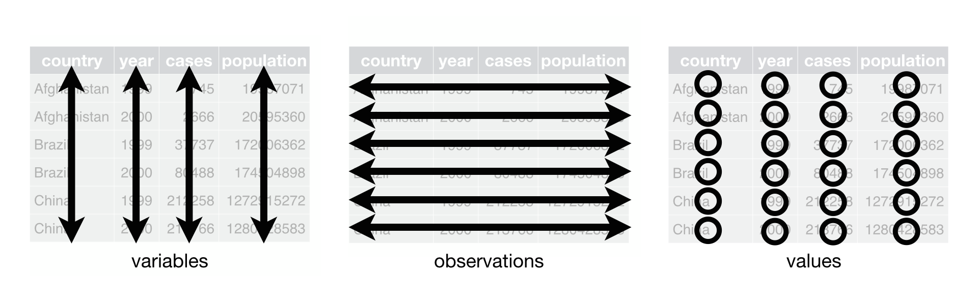
Basic concepts

1. Each variable must have its own column.
2. Each observation must have its own row.
3. Each value must have its own cell.

Load necessary libraries

library("readxl") # Import the data from Excel file
library("readr")  # Import the data from Excel file

library("dplyr")  # filter and reformat data frames
library("tidyr")  # make data tidy

library("stringr") # manipulate strings
library("lubridate") # manipulate date 

library("ggplot2") # graphics

Read and Write data

Oceanographic data

CARBOM cruise off Brazil

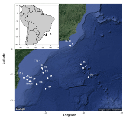
• Stations
• Depth
• Coordinates
• Temperature, Salinity
• Nitrates, Phosphates

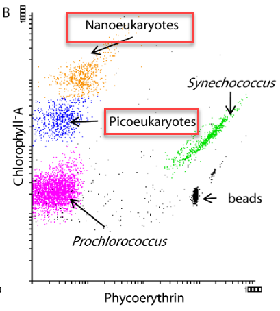
Microbial populations

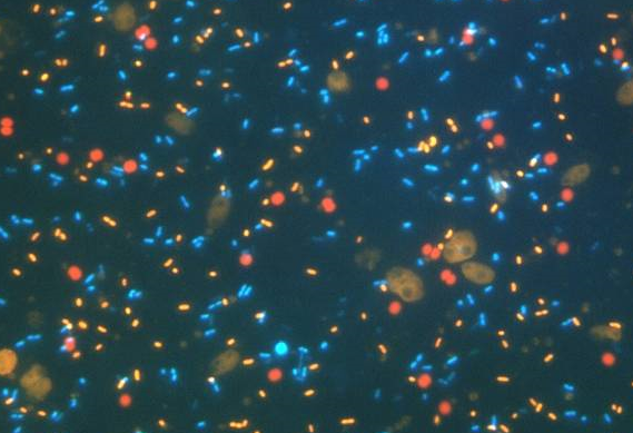
• Flow cytometry :
  • pico-eukaryotes
  • nano-eukaryotes

Read data

Text file - TAB delimited

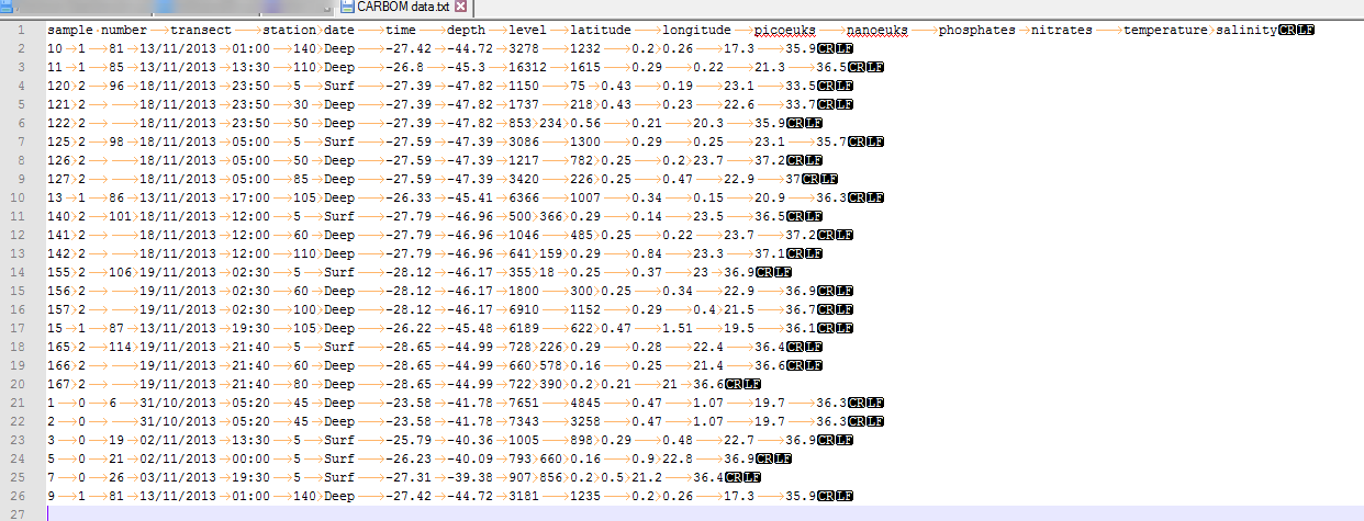
Reading a text file

  samples <- readr::read_tsv("data/CARBOM data.txt")

sample number	transect	station	date	time	depth	level	latitude	longitude	picoeuks	nanoeuks	phosphates	nitrates	temperature	salinity
10	1	81	13/11/2013	01:00:00	140	Deep	-27.42	-44.72	3278	1232	0.20	0.26	17.3	35.9
11	1	85	13/11/2013	13:30:00	110	Deep	-26.80	-45.30	16312	1615	0.29	0.22	21.3	36.5
120	2	96	18/11/2013	23:50:00	5	Surf	-27.39	-47.82	1150	75	0.43	0.19	23.1	33.5
121	2		18/11/2013	23:50:00	30	Deep	-27.39	-47.82	1737	218	0.43	0.23	22.6	33.7
122	2		18/11/2013	23:50:00	50	Deep	-27.39	-47.82	853	234	0.56	0.21	20.3	35.9
125	2	98	18/11/2013	05:00:00	5	Surf	-27.59	-47.39	3086	1300	0.29	0.25	23.1	35.7
126	2		18/11/2013	05:00:00	50	Deep	-27.59	-47.39	1217	782	0.25	0.20	23.7	37.2
127	2		18/11/2013	05:00:00	85	Deep	-27.59	-47.39	3420	226	0.25	0.47	22.9	37.0
13	1	86	13/11/2013	17:00:00	105	Deep	-26.33	-45.41	6366	1007	0.34	0.15	20.9	36.3
140	2	101	18/11/2013	12:00:00	5	Surf	-27.79	-46.96	500	366	0.29	0.14	23.5	36.5

• readr::read_tsv() : read tab delimited files

• readr::read_csv() : read comma delimited files

• readr::write_tsv() : write tab delimited files

Excel sheet

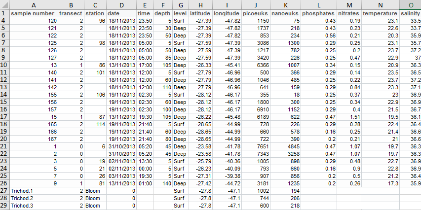
Read the data - read_excel

  samples <- readxl::read_excel("data/CARBOM data.xlsx", 
                           sheet = "Samples_boat")

sample number	transect	station	date	time	depth	level	latitude	longitude	picoeuks	nanoeuks	phosphates	nitrates	temperature	salinity
10	1	81	2013-11-13	1899-12-31 01:00:00	140	Deep	-27.42	-44.72	3278	1232	0.20	0.26	17.3	35.9
11	1	85	2013-11-13	1899-12-31 13:30:00	110	Deep	-26.80	-45.30	16312	1615	0.29	0.22	21.3	36.5
120	2	96	2013-11-18	1899-12-31 23:50:00	5	Surf	-27.39	-47.82	1150	75	0.43	0.19	23.1	33.5
121	2		2013-11-18	1899-12-31 23:50:00	30	Deep	-27.39	-47.82	1737	218	0.43	0.23	22.6	33.7
122	2		2013-11-18	1899-12-31 23:50:00	50	Deep	-27.39	-47.82	853	234	0.56	0.21	20.3	35.9
125	2	98	2013-11-18	1899-12-31 05:00:00	5	Surf	-27.59	-47.39	3086	1300	0.29	0.25	23.1	35.7
126	2		2013-11-18	1899-12-31 05:00:00	50	Deep	-27.59	-47.39	1217	782	0.25	0.20	23.7	37.2
127	2		2013-11-18	1899-12-31 05:00:00	85	Deep	-27.59	-47.39	3420	226	0.25	0.47	22.9	37.0
13	1	86	2013-11-13	1899-12-31 17:00:00	105	Deep	-26.33	-45.41	6366	1007	0.34	0.15	20.9	36.3
140	2	101	2013-11-18	1899-12-31 12:00:00	5	Surf	-27.79	-46.96	500	366	0.29	0.14	23.5	36.5

• Can also select a range : e.g. A1:Q26
• Can skip lines

Bad data input under Excel

sample number	transect	station	date	time	depth	level	latitude	longitude	picoeuks	nanoeuks	phosphates	nitrates	temperature	salinity
10	1	81	2013-11-13	1899-12-31 01:00:00	140	Deep	-27.42	-44.72	3278	1232	0.20	0.26	17.3	35.9
11	1	85	2013-11-13	1899-12-31 13:30:00	110	Deep	-26.80	-45.30	16312	1615	0.29	0.22	21.3	36.5
120	2	96	2013-11-18	1899-12-31 23:50:00	5	Surf	-27.39	-47.82	1150	75	0.43	0.19	23.1	33.5
121	2		2013-11-18	1899-12-31 23:50:00	30	Deep	-27.39	-47.82	1737	218	0.43	0.23	22.6	33.7
122	2		2013-11-18	1899-12-31 23:50:00	50	Deep	-27.39	-47.82	853	234	0.56	0.21	20.3	35.9
125	2	98	2013-11-18	1899-12-31 05:00:00	5	Surf	-27.59	-47.39	3086	1300	0.29	0.25	23.1	35.7
126	2		2013-11-18	1899-12-31 05:00:00	50	Deep	-27.59	-47.39	1217	782	0.25	0.20	23.7	37.2
127	2		2013-11-18	1899-12-31 05:00:00	85	Deep	-27.59	-47.39	3420	226	0.25	0.47	22.9	37.0
13	1	86	2013-11-13	1899-12-31 17:00:00	105	Deep	-26.33	-45.41	6366	1007	0.34	0.15	20.9	36.3
140	2	101	2013-11-18	1899-12-31 12:00:00	5	Surf	-27.79	-46.96	500	366	0.29	0.14	23.5	36.5

• There are missing values in the column station because only recorded when changed

Filling missing values - fill

  samples <- tidyr::fill(samples, station)

sample number	transect	station	date	time	depth	level	latitude	longitude	picoeuks	nanoeuks	phosphates	nitrates	temperature	salinity
10	1	81	2013-11-13	1899-12-31 01:00:00	140	Deep	-27.42	-44.72	3278	1232	0.20	0.26	17.3	35.9
11	1	85	2013-11-13	1899-12-31 13:30:00	110	Deep	-26.80	-45.30	16312	1615	0.29	0.22	21.3	36.5
120	2	96	2013-11-18	1899-12-31 23:50:00	5	Surf	-27.39	-47.82	1150	75	0.43	0.19	23.1	33.5
121	2	96	2013-11-18	1899-12-31 23:50:00	30	Deep	-27.39	-47.82	1737	218	0.43	0.23	22.6	33.7
122	2	96	2013-11-18	1899-12-31 23:50:00	50	Deep	-27.39	-47.82	853	234	0.56	0.21	20.3	35.9
125	2	98	2013-11-18	1899-12-31 05:00:00	5	Surf	-27.59	-47.39	3086	1300	0.29	0.25	23.1	35.7
126	2	98	2013-11-18	1899-12-31 05:00:00	50	Deep	-27.59	-47.39	1217	782	0.25	0.20	23.7	37.2
127	2	98	2013-11-18	1899-12-31 05:00:00	85	Deep	-27.59	-47.39	3420	226	0.25	0.47	22.9	37.0
13	1	86	2013-11-13	1899-12-31 17:00:00	105	Deep	-26.33	-45.41	6366	1007	0.34	0.15	20.9	36.3
140	2	101	2013-11-18	1899-12-31 12:00:00	5	Surf	-27.79	-46.96	500	366	0.29	0.14	23.5	36.5

• All missing values have been filled in.

Write data

Text file

• readr::write_tsv() : write tab delimited files

  readr::write_tsv(samples, "data/CARBOM data fixed.tsv")

Excel file

• openxlsx::write.xlsx : write tab delimited files

• Many options: specific sheet, formatting etc…

  openxlsx::write.xlsx(samples, "data/CARBOM data fixed.xlsx")

Write data

Library rio

• Many output formats
• import() / export()

dplyr - Manipulate tables

@allison_horst

Manipulate columns

List and Summarize columns

List columns

  colnames(samples)

 [1] "sample number" "transect"      "station"       "date"         
 [5] "time"          "depth"         "level"         "latitude"     
 [9] "longitude"     "picoeuks"      "nanoeuks"      "phosphates"   
[13] "nitrates"      "temperature"   "salinity"     

Summarize columns

  summary(samples$depth)

   Min. 1st Qu.  Median    Mean 3rd Qu.    Max.    NA's 
    5.0     5.0    50.0    56.6   100.0   140.0       3 

Select specific columns - select

samples_select <- dplyr::select(samples, transect, `sample number`,
                                 station, depth, latitude, longitude, 
                                 picoeuks, nanoeuks)

transect	sample number	station	depth	latitude	longitude	picoeuks	nanoeuks
1	10	81	140	-27.42	-44.72	3278	1232
1	11	85	110	-26.80	-45.30	16312	1615
2	120	96	5	-27.39	-47.82	1150	75
2	121	96	30	-27.39	-47.82	1737	218
2	122	96	50	-27.39	-47.82	853	234
2	125	98	5	-27.59	-47.39	3086	1300
2	126	98	50	-27.59	-47.39	1217	782
2	127	98	85	-27.59	-47.39	3420	226
1	13	86	105	-26.33	-45.41	6366	1007
2	140	101	5	-27.79	-46.96	500	366

* Column names are not “quoted” (in base R you need to “quote” the column names)

* Better not to put space in column header because then must enclose column name with ` (back-quote)

Select a range of columns - select

  samples_select <- dplyr::select(samples, transect:nanoeuks)

transect	station	date	time	depth	level	latitude	longitude	picoeuks	nanoeuks
1	81	2013-11-13	1899-12-31 01:00:00	140	Deep	-27.42	-44.72	3278	1232
1	85	2013-11-13	1899-12-31 13:30:00	110	Deep	-26.80	-45.30	16312	1615
2	96	2013-11-18	1899-12-31 23:50:00	5	Surf	-27.39	-47.82	1150	75
2	96	2013-11-18	1899-12-31 23:50:00	30	Deep	-27.39	-47.82	1737	218
2	96	2013-11-18	1899-12-31 23:50:00	50	Deep	-27.39	-47.82	853	234
2	98	2013-11-18	1899-12-31 05:00:00	5	Surf	-27.59	-47.39	3086	1300
2	98	2013-11-18	1899-12-31 05:00:00	50	Deep	-27.59	-47.39	1217	782
2	98	2013-11-18	1899-12-31 05:00:00	85	Deep	-27.59	-47.39	3420	226
1	86	2013-11-13	1899-12-31 17:00:00	105	Deep	-26.33	-45.41	6366	1007
2	101	2013-11-18	1899-12-31 12:00:00	5	Surf	-27.79	-46.96	500	366

Unselect columns - select

  samples_select <- dplyr::select (samples, -nitrates, -phosphates)

sample number	transect	station	date	time	depth	level	latitude	longitude	picoeuks	nanoeuks	temperature	salinity
10	1	81	2013-11-13	1899-12-31 01:00:00	140	Deep	-27.42	-44.72	3278	1232	17.3	35.9
11	1	85	2013-11-13	1899-12-31 13:30:00	110	Deep	-26.80	-45.30	16312	1615	21.3	36.5
120	2	96	2013-11-18	1899-12-31 23:50:00	5	Surf	-27.39	-47.82	1150	75	23.1	33.5
121	2	96	2013-11-18	1899-12-31 23:50:00	30	Deep	-27.39	-47.82	1737	218	22.6	33.7
122	2	96	2013-11-18	1899-12-31 23:50:00	50	Deep	-27.39	-47.82	853	234	20.3	35.9
125	2	98	2013-11-18	1899-12-31 05:00:00	5	Surf	-27.59	-47.39	3086	1300	23.1	35.7
126	2	98	2013-11-18	1899-12-31 05:00:00	50	Deep	-27.59	-47.39	1217	782	23.7	37.2
127	2	98	2013-11-18	1899-12-31 05:00:00	85	Deep	-27.59	-47.39	3420	226	22.9	37.0
13	1	86	2013-11-13	1899-12-31 17:00:00	105	Deep	-26.33	-45.41	6366	1007	20.9	36.3
140	2	101	2013-11-18	1899-12-31 12:00:00	5	Surf	-27.79	-46.96	500	366	23.5	36.5

Using the pipe operator - %>%

  samples_select <- samples %>% dplyr::select(transect:nanoeuks)

transect	station	date	time	depth	level	latitude	longitude	picoeuks	nanoeuks
1	81	2013-11-13	1899-12-31 01:00:00	140	Deep	-27.42	-44.72	3278	1232
1	85	2013-11-13	1899-12-31 13:30:00	110	Deep	-26.80	-45.30	16312	1615
2	96	2013-11-18	1899-12-31 23:50:00	5	Surf	-27.39	-47.82	1150	75
2	96	2013-11-18	1899-12-31 23:50:00	30	Deep	-27.39	-47.82	1737	218
2	96	2013-11-18	1899-12-31 23:50:00	50	Deep	-27.39	-47.82	853	234
2	98	2013-11-18	1899-12-31 05:00:00	5	Surf	-27.59	-47.39	3086	1300
2	98	2013-11-18	1899-12-31 05:00:00	50	Deep	-27.59	-47.39	1217	782
2	98	2013-11-18	1899-12-31 05:00:00	85	Deep	-27.59	-47.39	3420	226
1	86	2013-11-13	1899-12-31 17:00:00	105	Deep	-26.33	-45.41	6366	1007
2	101	2013-11-18	1899-12-31 12:00:00	5	Surf	-27.79	-46.96	500	366

• It is cleaner to write on 2 lines

  samples_select <- samples %>% 
    dplyr::select(transect:nanoeuks)

Renaming variables - rename

  samples <- samples %>% 
    dplyr::rename(sample_number = `sample number`)

sample_number	transect	station	date	time	depth	level	latitude	longitude	picoeuks	nanoeuks	phosphates	nitrates	temperature	salinity
10	1	81	2013-11-13	1899-12-31 01:00:00	140	Deep	-27.42	-44.72	3278	1232	0.20	0.26	17.3	35.9
11	1	85	2013-11-13	1899-12-31 13:30:00	110	Deep	-26.80	-45.30	16312	1615	0.29	0.22	21.3	36.5
120	2	96	2013-11-18	1899-12-31 23:50:00	5	Surf	-27.39	-47.82	1150	75	0.43	0.19	23.1	33.5
121	2	96	2013-11-18	1899-12-31 23:50:00	30	Deep	-27.39	-47.82	1737	218	0.43	0.23	22.6	33.7
122	2	96	2013-11-18	1899-12-31 23:50:00	50	Deep	-27.39	-47.82	853	234	0.56	0.21	20.3	35.9
125	2	98	2013-11-18	1899-12-31 05:00:00	5	Surf	-27.59	-47.39	3086	1300	0.29	0.25	23.1	35.7
126	2	98	2013-11-18	1899-12-31 05:00:00	50	Deep	-27.59	-47.39	1217	782	0.25	0.20	23.7	37.2
127	2	98	2013-11-18	1899-12-31 05:00:00	85	Deep	-27.59	-47.39	3420	226	0.25	0.47	22.9	37.0
13	1	86	2013-11-13	1899-12-31 17:00:00	105	Deep	-26.33	-45.41	6366	1007	0.34	0.15	20.9	36.3
140	2	101	2013-11-18	1899-12-31 12:00:00	5	Surf	-27.79	-46.96	500	366	0.29	0.14	23.5	36.5

Creating new variables - mutate

  samples <- samples %>% 
    dplyr::mutate(pico_pct = picoeuks/(picoeuks+nanoeuks)*100)

sample_number	transect	station	date	time	depth	level	latitude	longitude	picoeuks	nanoeuks	phosphates	nitrates	temperature	salinity	pico_pct
10	1	81	2013-11-13	1899-12-31 01:00:00	140	Deep	-27.42	-44.72	3278	1232	0.20	0.26	17.3	35.9	72.68293
11	1	85	2013-11-13	1899-12-31 13:30:00	110	Deep	-26.80	-45.30	16312	1615	0.29	0.22	21.3	36.5	90.99124
120	2	96	2013-11-18	1899-12-31 23:50:00	5	Surf	-27.39	-47.82	1150	75	0.43	0.19	23.1	33.5	93.87755
121	2	96	2013-11-18	1899-12-31 23:50:00	30	Deep	-27.39	-47.82	1737	218	0.43	0.23	22.6	33.7	88.84910
122	2	96	2013-11-18	1899-12-31 23:50:00	50	Deep	-27.39	-47.82	853	234	0.56	0.21	20.3	35.9	78.47286
125	2	98	2013-11-18	1899-12-31 05:00:00	5	Surf	-27.59	-47.39	3086	1300	0.29	0.25	23.1	35.7	70.36024
126	2	98	2013-11-18	1899-12-31 05:00:00	50	Deep	-27.59	-47.39	1217	782	0.25	0.20	23.7	37.2	60.88044
127	2	98	2013-11-18	1899-12-31 05:00:00	85	Deep	-27.59	-47.39	3420	226	0.25	0.47	22.9	37.0	93.80143
13	1	86	2013-11-13	1899-12-31 17:00:00	105	Deep	-26.33	-45.41	6366	1007	0.34	0.15	20.9	36.3	86.34206
140	2	101	2013-11-18	1899-12-31 12:00:00	5	Surf	-27.79	-46.96	500	366	0.29	0.14	23.5	36.5	57.73672

• You can also use transmute() but then it will drop all the other columns.
• It is much much better to compute new variables in R than in Excel, because you can easily track and correct errors.

Using the pipe operator you can chain operations

  samples_select <- samples  %>% 
    dplyr::select(sample_number:nanoeuks, level) %>% 
    dplyr::mutate(pico_pct = picoeuks/(picoeuks+nanoeuks)*100)

sample_number	transect	station	date	time	depth	level	latitude	longitude	picoeuks	nanoeuks	pico_pct
10	1	81	2013-11-13	1899-12-31 01:00:00	140	Deep	-27.42	-44.72	3278	1232	72.68293
11	1	85	2013-11-13	1899-12-31 13:30:00	110	Deep	-26.80	-45.30	16312	1615	90.99124
120	2	96	2013-11-18	1899-12-31 23:50:00	5	Surf	-27.39	-47.82	1150	75	93.87755
121	2	96	2013-11-18	1899-12-31 23:50:00	30	Deep	-27.39	-47.82	1737	218	88.84910
122	2	96	2013-11-18	1899-12-31 23:50:00	50	Deep	-27.39	-47.82	853	234	78.47286
125	2	98	2013-11-18	1899-12-31 05:00:00	5	Surf	-27.59	-47.39	3086	1300	70.36024
126	2	98	2013-11-18	1899-12-31 05:00:00	50	Deep	-27.59	-47.39	1217	782	60.88044
127	2	98	2013-11-18	1899-12-31 05:00:00	85	Deep	-27.59	-47.39	3420	226	93.80143
13	1	86	2013-11-13	1899-12-31 17:00:00	105	Deep	-26.33	-45.41	6366	1007	86.34206
140	2	101	2013-11-18	1899-12-31 12:00:00	5	Surf	-27.79	-46.96	500	366	57.73672

Creating labels with mutate and stringr functions

  samples <- samples %>% 
    dplyr::mutate(sample_label = str_c("TR",transect,"St",station, sep="_"))

sample_number	transect	station	date	time	sample_label
10	1	81	2013-11-13	1899-12-31 01:00:00	TR_1_St_81
11	1	85	2013-11-13	1899-12-31 13:30:00	TR_1_St_85
120	2	96	2013-11-18	1899-12-31 23:50:00	TR_2_St_96
121	2	96	2013-11-18	1899-12-31 23:50:00	TR_2_St_96
122	2	96	2013-11-18	1899-12-31 23:50:00	TR_2_St_96
125	2	98	2013-11-18	1899-12-31 05:00:00	TR_2_St_98
126	2	98	2013-11-18	1899-12-31 05:00:00	TR_2_St_98
127	2	98	2013-11-18	1899-12-31 05:00:00	TR_2_St_98
13	1	86	2013-11-13	1899-12-31 17:00:00	TR_1_St_86
140	2	101	2013-11-18	1899-12-31 12:00:00	TR_2_St_101

Changing type of some columns - mutate

• Use the lubridate package to manipulate dates

  samples <- samples %>% 
    dplyr::mutate(time = str_c(lubridate::hour(time), 
                               lubridate::minute(time), sep=":"))

sample_number	transect	station	date	time	depth	level	latitude	longitude	picoeuks	nanoeuks	phosphates	nitrates	temperature	salinity	pico_pct
10	1	81	2013-11-13	1:0	140	Deep	-27.42	-44.72	3278	1232	0.20	0.26	17.3	35.9	72.68293
11	1	85	2013-11-13	13:30	110	Deep	-26.80	-45.30	16312	1615	0.29	0.22	21.3	36.5	90.99124
120	2	96	2013-11-18	23:50	5	Surf	-27.39	-47.82	1150	75	0.43	0.19	23.1	33.5	93.87755
121	2	96	2013-11-18	23:50	30	Deep	-27.39	-47.82	1737	218	0.43	0.23	22.6	33.7	88.84910
122	2	96	2013-11-18	23:50	50	Deep	-27.39	-47.82	853	234	0.56	0.21	20.3	35.9	78.47286
125	2	98	2013-11-18	5:0	5	Surf	-27.59	-47.39	3086	1300	0.29	0.25	23.1	35.7	70.36024
126	2	98	2013-11-18	5:0	50	Deep	-27.59	-47.39	1217	782	0.25	0.20	23.7	37.2	60.88044
127	2	98	2013-11-18	5:0	85	Deep	-27.59	-47.39	3420	226	0.25	0.47	22.9	37.0	93.80143
13	1	86	2013-11-13	17:0	105	Deep	-26.33	-45.41	6366	1007	0.34	0.15	20.9	36.3	86.34206
140	2	101	2013-11-18	12:0	5	Surf	-27.79	-46.96	500	366	0.29	0.14	23.5	36.5	57.73672

Manipulating rows

Order rows - arrange

  samples <- samples %>% 
    dplyr::arrange(transect, station)

sample_number	transect	station	date	time	depth	level	latitude	longitude	picoeuks	nanoeuks	phosphates	nitrates	temperature	salinity	pico_pct
3	0	19	2013-11-02	13:30	5	Surf	-25.79	-40.36	1005	898	0.29	0.48	22.7	36.9	52.81135
5	0	21	2013-11-02	0:0	5	Surf	-26.23	-40.09	793	660	0.16	0.90	22.8	36.9	54.57674
7	0	26	2013-11-03	19:30	5	Surf	-27.31	-39.38	907	856	0.20	0.50	21.2	36.4	51.44640
1	0	6	2013-10-31	5:20	45	Deep	-23.58	-41.78	7651	4845	0.47	1.07	19.7	36.3	61.22759
2	0	6	2013-10-31	5:20	45	Deep	-23.58	-41.78	7343	3258	0.47	1.07	19.7	36.3	69.26705
10	1	81	2013-11-13	1:0	140	Deep	-27.42	-44.72	3278	1232	0.20	0.26	17.3	35.9	72.68293
9	1	81	2013-11-13	1:0	140	Deep	-27.42	-44.72	3181	1235	0.20	0.26	17.3	35.9	72.03351
11	1	85	2013-11-13	13:30	110	Deep	-26.80	-45.30	16312	1615	0.29	0.22	21.3	36.5	90.99124
13	1	86	2013-11-13	17:0	105	Deep	-26.33	-45.41	6366	1007	0.34	0.15	20.9	36.3	86.34206
15	1	87	2013-11-13	19:30	105	Deep	-26.22	-45.48	6189	622	0.47	1.51	19.5	36.1	90.86771

• Station 6 is not ordered numerically. It is because station is a character column.

Order rows - transform to numeric

  samples <- samples %>% 
    dplyr::mutate(station = as.numeric(station)) %>% 
    dplyr::arrange(transect, station)

sample_number	transect	station	date	time	depth	level	latitude	longitude	picoeuks	nanoeuks	phosphates	nitrates	temperature	salinity	pico_pct
1	0	6	2013-10-31	5:20	45	Deep	-23.58	-41.78	7651	4845	0.47	1.07	19.7	36.3	61.22759
2	0	6	2013-10-31	5:20	45	Deep	-23.58	-41.78	7343	3258	0.47	1.07	19.7	36.3	69.26705
3	0	19	2013-11-02	13:30	5	Surf	-25.79	-40.36	1005	898	0.29	0.48	22.7	36.9	52.81135
5	0	21	2013-11-02	0:0	5	Surf	-26.23	-40.09	793	660	0.16	0.90	22.8	36.9	54.57674
7	0	26	2013-11-03	19:30	5	Surf	-27.31	-39.38	907	856	0.20	0.50	21.2	36.4	51.44640
10	1	81	2013-11-13	1:0	140	Deep	-27.42	-44.72	3278	1232	0.20	0.26	17.3	35.9	72.68293
9	1	81	2013-11-13	1:0	140	Deep	-27.42	-44.72	3181	1235	0.20	0.26	17.3	35.9	72.03351
11	1	85	2013-11-13	13:30	110	Deep	-26.80	-45.30	16312	1615	0.29	0.22	21.3	36.5	90.99124
13	1	86	2013-11-13	17:0	105	Deep	-26.33	-45.41	6366	1007	0.34	0.15	20.9	36.3	86.34206
15	1	87	2013-11-13	19:30	105	Deep	-26.22	-45.48	6189	622	0.47	1.51	19.5	36.1	90.86771

• One station named “Bloom” could not be converted to numerical (-> NA)

Summarize rows - count

• Compute number of stations per transect

  stations_count <- samples %>% 
    dplyr::count(transect) 

transect	n
0	5
1	5
2	18

Summarize rows - group_by / summarize

• Group by transect and station
• Compute mean of the percent picoplankton

  samples_mean <- samples %>% 
    dplyr::group_by(transect, station) %>% 
    dplyr::summarise(n_samples = n(), 
              mean_pico_percent = mean(pico_pct, na.rm=TRUE))

transect	station	n_samples	mean_pico_percent
0	6	2	65.24732
0	19	1	52.81135
0	21	1	54.57674
0	26	1	51.44640
1	81	2	72.35822
1	85	1	90.99124
1	86	1	86.34206
1	87	1	90.86771
2	96	3	87.06651
2	98	3	75.01403

Filtering rows - filter

• Get only the surface samples

  samples_surf <- samples %>% 
    dplyr::filter(level == "Surf" ) 

sample_number	transect	station	date	time	depth	level	latitude	longitude	picoeuks	nanoeuks	phosphates	nitrates	temperature	salinity	pico_pct
3	0	19	2013-11-02	13:30	5	Surf	-25.79	-40.36	1005	898	0.29	0.48	22.7	36.9	52.81135
5	0	21	2013-11-02	0:0	5	Surf	-26.23	-40.09	793	660	0.16	0.90	22.8	36.9	54.57674
7	0	26	2013-11-03	19:30	5	Surf	-27.31	-39.38	907	856	0.20	0.50	21.2	36.4	51.44640
120	2	96	2013-11-18	23:50	5	Surf	-27.39	-47.82	1150	75	0.43	0.19	23.1	33.5	93.87755
125	2	98	2013-11-18	5:0	5	Surf	-27.59	-47.39	3086	1300	0.29	0.25	23.1	35.7	70.36024
140	2	101	2013-11-18	12:0	5	Surf	-27.79	-46.96	500	366	0.29	0.14	23.5	36.5	57.73672
155	2	106	2013-11-19	2:30	5	Surf	-28.12	-46.17	355	18	0.25	0.37	23.0	36.9	95.17426
165	2	114	2013-11-19	21:40	5	Surf	-28.65	-44.99	728	226	0.29	0.28	22.4	36.4	76.31027
Trichod.1	2					Surf	-27.80	-47.10	1002	194					83.77926
Trichod.2	2					Surf	-27.80	-47.10	744	206					78.31579

• ! Use the logical operators == != > >= < <= is.na()

Recap

• Import and Export data

• Select and create columns

• Summarize data

• Joining

• Long vs. Wide format

• Displaying tables

Next time: Data visualization (ggplot2)

• Understand the “grammar” of graphics
• Create exploratory graphics

Reading list

• Chapter 28 of R for data science
• Fundamental of data visualization
• Data visualization: practical introduction