R course
Daniel Vaulot
2023-01-19
![]()
![]()
![]()
![]()
Introduction to R
Introduction
![]()
- If you are an R guru:
- Please refrain to answer during this session…
- Help your neighbor
- Two special slide formatting
- Your turn…
- Warning
History of computer languages

History of R
![]()
Mid 1970s - S Language for Statistical Computing conceived by John Chambers, Rick Becker, Trevor Hastie, Allan Wilks and others at Bell Labs
Early 1990’s - R was first implemented in the early 1990’s by Robert Gentleman and Ross Ihaka, both faculty members at the University of Auckland.
1995 - Open Source Project
1997 - Managed by the R Core Group
2000 - First release of R
2011 - First release of R studio
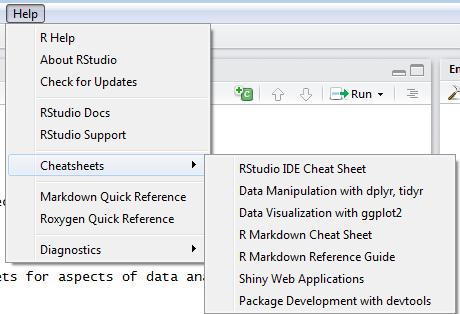
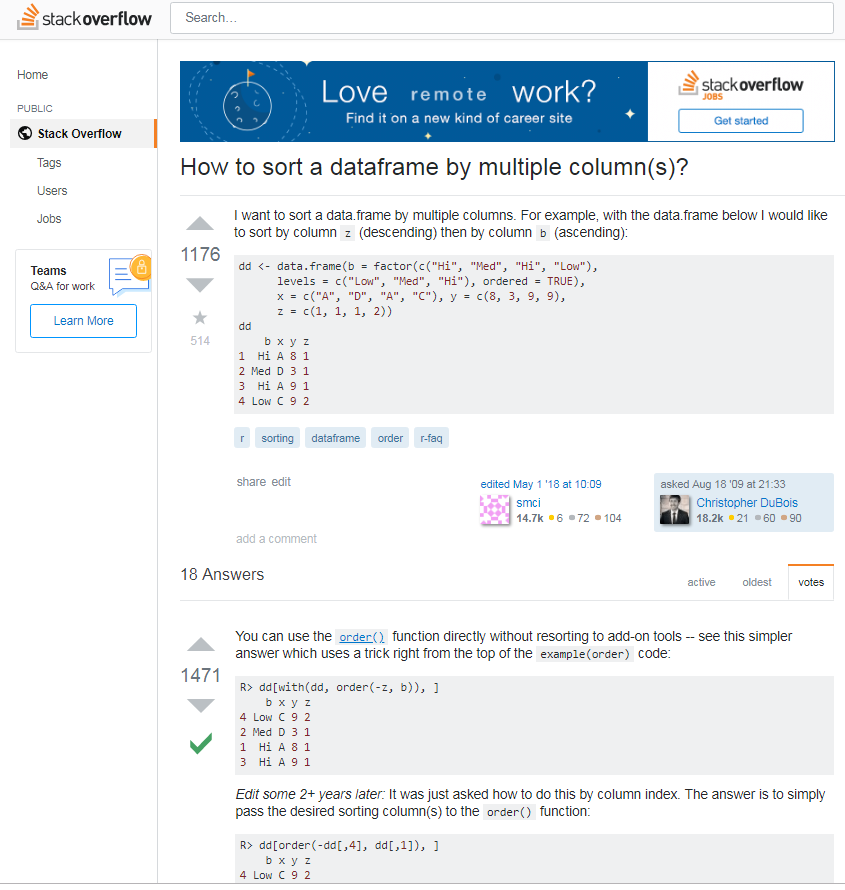
Help
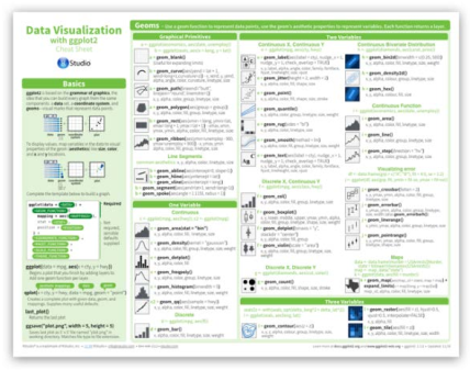
Cheat sheets
The R studio interface
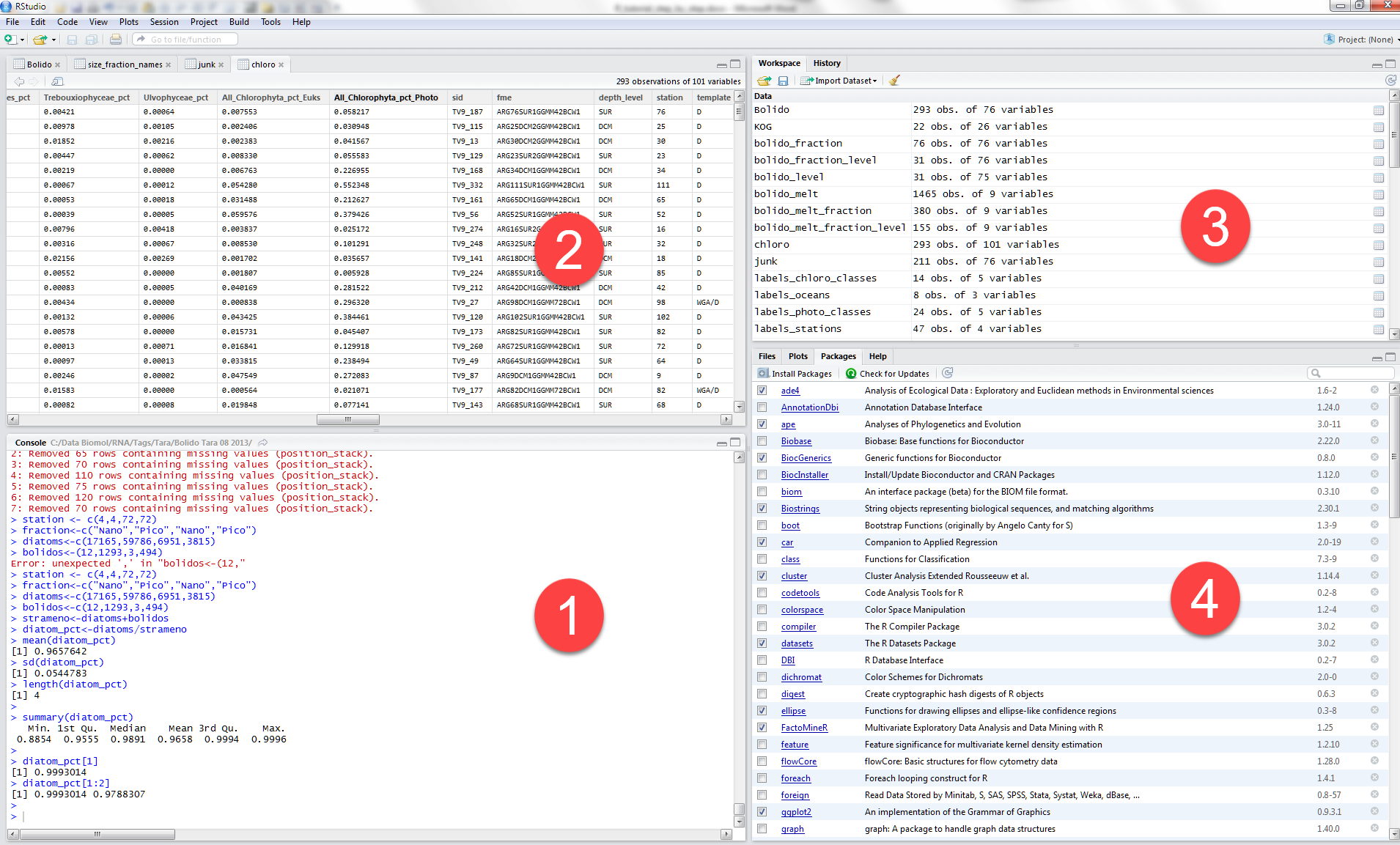
- Bottom left
- Console
- Top left
- File editor for .R and .Rmd files
- Data frame visualization
- Top right
- Environment (i.e. R objects)
- History
- Bottom right
- Files
- Plots
- Packages
- Help
Create a new project
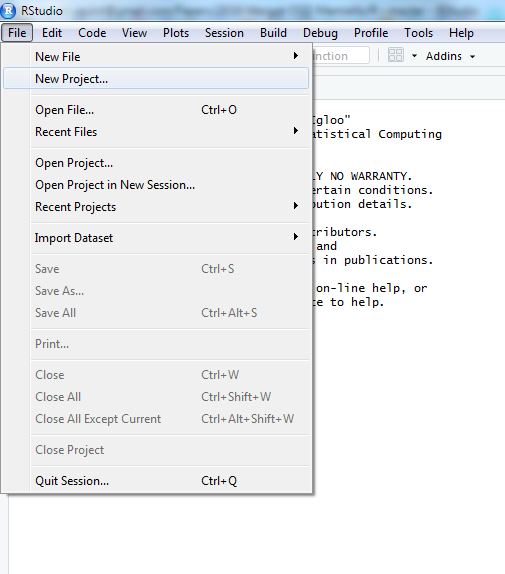
- Open R studio
- Create new project for the course in a new directory
- e.g.
Microbes course
- e.g.
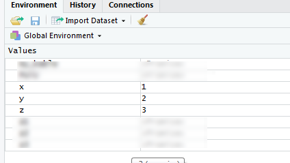
Visualizing objects
You can view the values of the objects in R-studio environment window (top-right)
Functions
Functions perform specific task on objects
- e.g. to concatanate strings we use paste()
paste(first,last)[1] "Jo Biden"Functions take arguments and return an object called result
To know the arguments
- Use “?”
- Can also go directly to Help panel and type function name
? paste() # Do not forget the parenthesis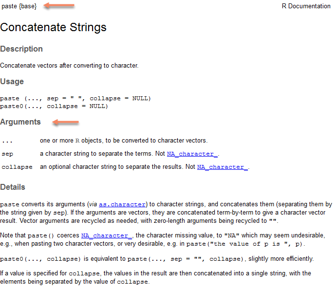

Plot
- Histogram
  library(graphics)
  hist(y)
What is this “library()”
Packages
Packages are set of functions that have a common goal.
They are really the strength of R
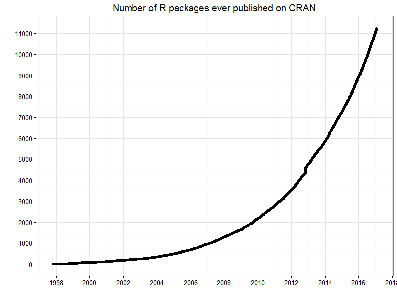
- And these are only the “official”” packages. You can find more on GitHub
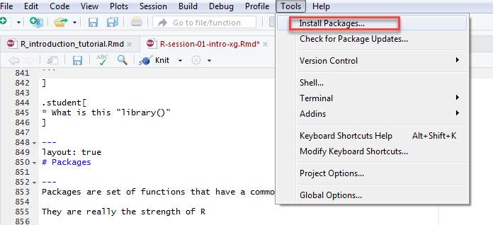
Installing a package
Download on your computer the package you need
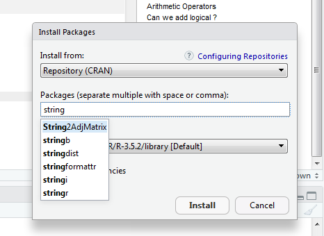
Install package stringr (to manipulate strings of characters)
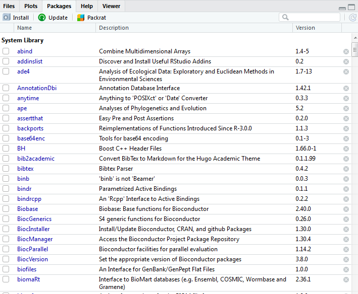
List installed packages
Next: 02 - Data wrangling
- Data frames
- Concept of tidy data
- Reading data
- Manipulating data
- Selecting columns
- Selecting rows