R course

Daniel Vaulot

2023-06-22

Data visualization

R - Session 03

Graph types
Grammar of graphics
Playing with ggplot2
Multiple graphs
ggplot2 syntax

Intro to Data vizualisation

Installation and Resources

Packages

ggplot2
patchwork

Download

R-session-03.zip

Reading

Chapter 28 of R for data science

Resources

Workflow

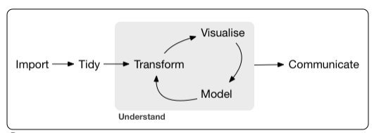
Graph purposes

Analysis graphs
- design to see patterns, trends
- aid the process of data description
- interpretation

Presentation graphs
- design to attract attention
- make a point
- illustrate a conclusion

Source: Michael Friendly

Graph types

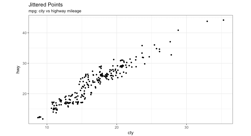
Jitter

Two variables numerical

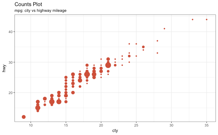
Bubble

Two variables numerical
Add another variable numerical

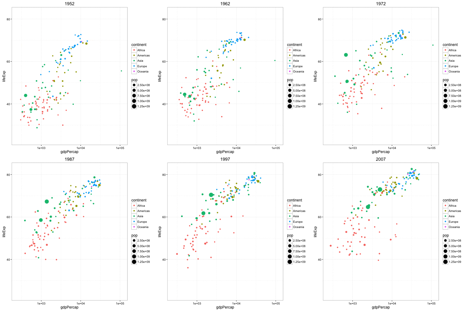
Animate

Two variables numerical
One variable numerical
One variable categorical
Animate another variable

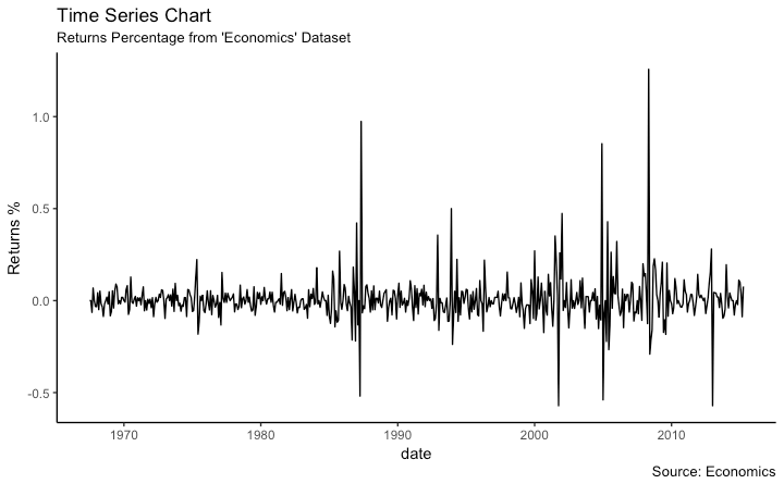
Times series

Line graph

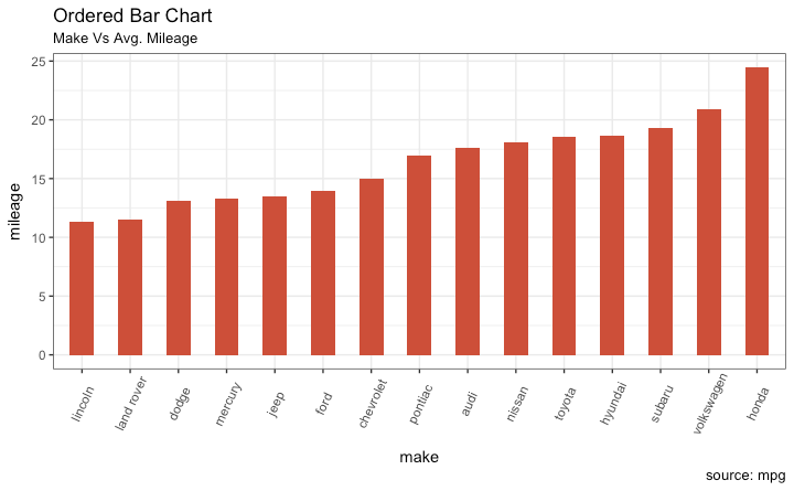
Bargraphs

One variable categorical
One variable numerical

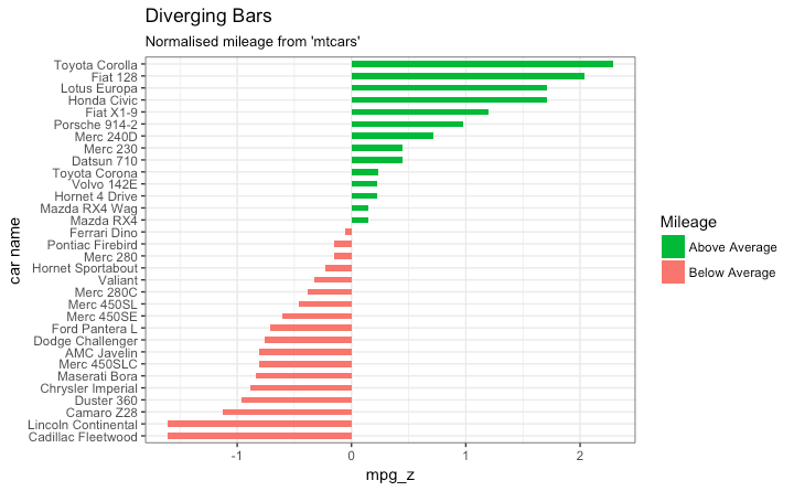
Bargraphs

Rotate

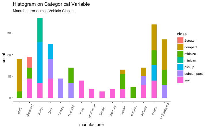
Bargraphs

Two variable categorical
One variable numerical

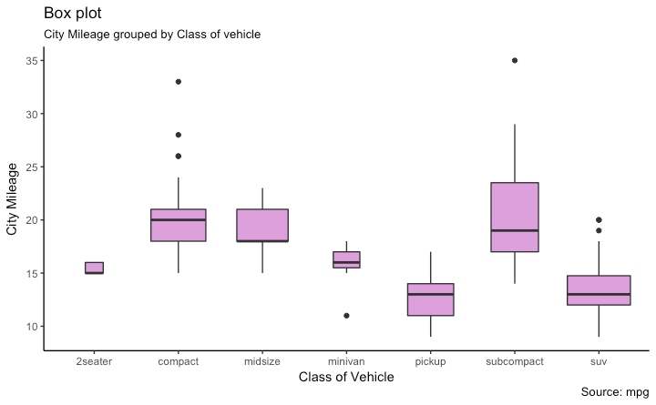
Boxplots

One variable categorical
One variable numerical but with many values

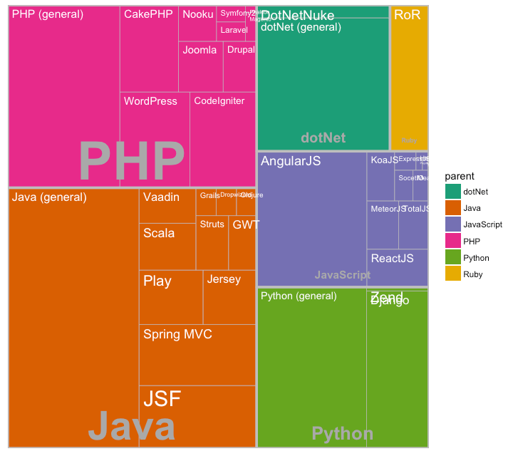
Treemaps

One variable categorical
One variable numerical
Much better than pie charts

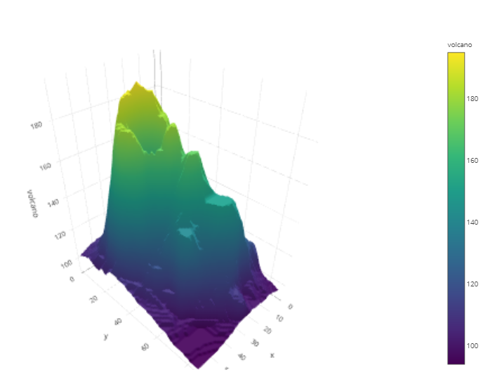
3D

Three variable numerical
Avoid unless it is a simple shape

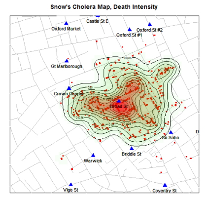
Contours

Three variable numerical
Better than 3D

Many…

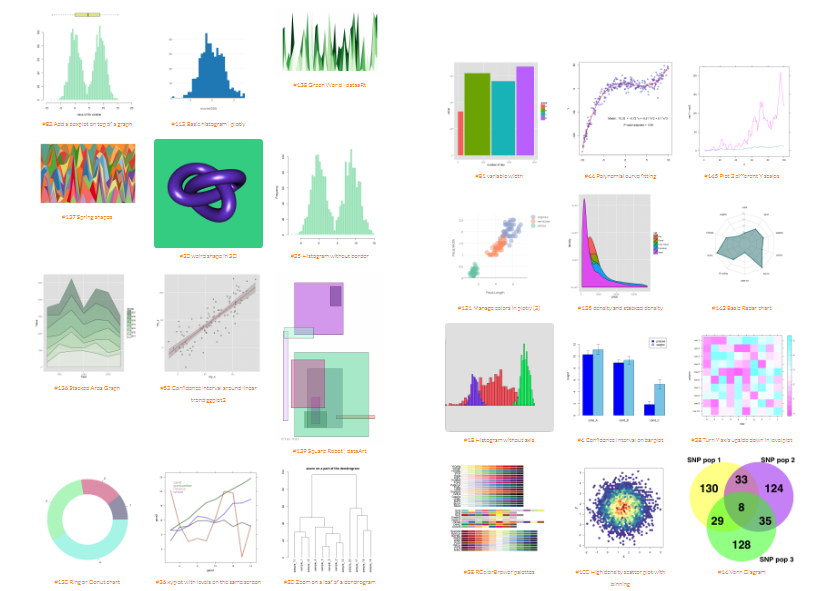
Choose as a function of what you want to analyze or the story you want to tell
https://www.r-graph-gallery.com/all-graphs/

ggplot2

Initialize

Load necessary libraries

library("readxl") # Import the data from Excel file
library("dplyr")  # filter and reformat data frames
library("ggplot2") # graphics
library("patchwork") # arrange graphics

Read the data

samples <- readxl::read_excel("data/CARBOM data.xlsx", 
                         sheet = "Samples_boat") %>% 
           tidyr::fill(station)

sample number	transect	station	date	time	depth	level	latitude	longitude	picoeuks	nanoeuks	phosphates	nitrates	temperature	salinity
10	1	81	2013-11-13	1899-12-31 01:00:00	140	Deep	-27.42	-44.72	3278	1232	0.20	0.26	17.3	35.9
11	1	85	2013-11-13	1899-12-31 13:30:00	110	Deep	-26.80	-45.30	16312	1615	0.29	0.22	21.3	36.5
120	2	96	2013-11-18	1899-12-31 23:50:00	5	Surf	-27.39	-47.82	1150	75	0.43	0.19	23.1	33.5
121	2	96	2013-11-18	1899-12-31 23:50:00	30	Deep	-27.39	-47.82	1737	218	0.43	0.23	22.6	33.7
122	2	96	2013-11-18	1899-12-31 23:50:00	50	Deep	-27.39	-47.82	853	234	0.56	0.21	20.3	35.9
125	2	98	2013-11-18	1899-12-31 05:00:00	5	Surf	-27.59	-47.39	3086	1300	0.29	0.25	23.1	35.7
126	2	98	2013-11-18	1899-12-31 05:00:00	50	Deep	-27.59	-47.39	1217	782	0.25	0.20	23.7	37.2
127	2	98	2013-11-18	1899-12-31 05:00:00	85	Deep	-27.59	-47.39	3420	226	0.25	0.47	22.9	37.0
13	1	86	2013-11-13	1899-12-31 17:00:00	105	Deep	-26.33	-45.41	6366	1007	0.34	0.15	20.9	36.3
140	2	101	2013-11-18	1899-12-31 12:00:00	5	Surf	-27.79	-46.96	500	366	0.29	0.14	23.5	36.5

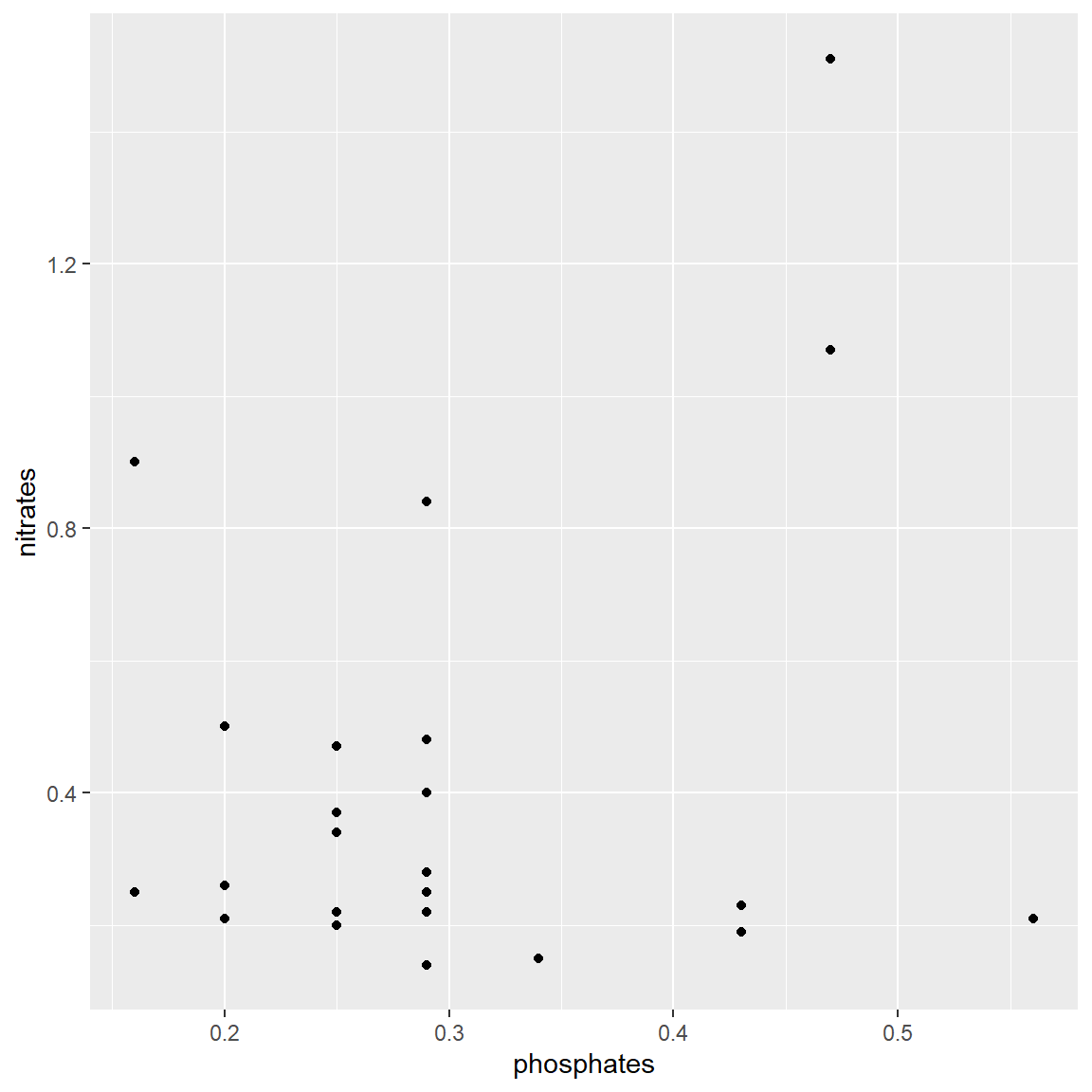
A simple plot

Choose the data set
Choose the geometric representation
Choose the aesthetics : x,y, color, shape etc…

# All functions are from ggplot2 
# package unless specified

ggplot(data=samples) + 
    geom_point(mapping = aes(x=phosphates, 
                            y=nitrates))

The grammar of graphics

 ggplot(data=samples) + 
  geom_point(mapping = aes(x=phosphates, 
                           y=nitrates))

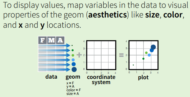
Every graph can be described as a combination of independent building blocks:

data: a data frame: quantitative, categorical; local or data base query
aesthetic mapping of variables into visual properties: size, color, x, y
geometric objects (“geom”): points, lines, areas, arrows, …
coordinate system (“coord”): Cartesian, log, polar, map

Alternatively

Move mapping into ggplot function

 ggplot(data=samples, 
        mapping = aes(x=phosphates, 
                      y=nitrates)) + 
  geom_point()

Alternatively

Remove function arguments

 ggplot(samples, 
        aes(x=phosphates, 
            y=nitrates)) + 
  geom_point()

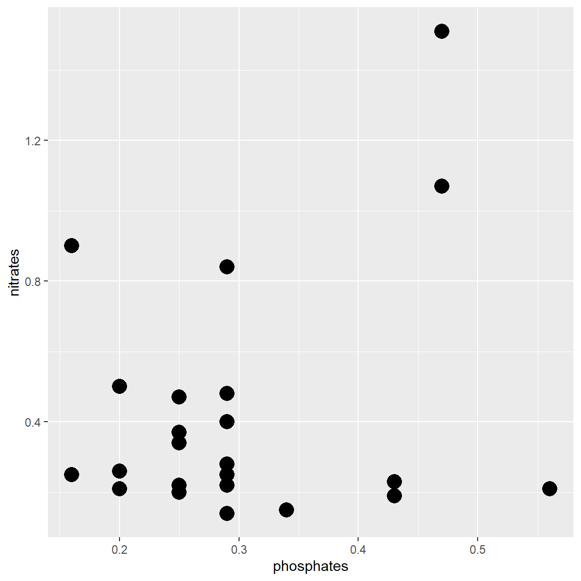
Makes dots bigger

Add: size=5 outside of the aesthetics function

 ggplot(samples,
        aes(x=phosphates, 
            y=nitrates)) + 
  geom_point(size=5)

Color according to depth level (discrete)

The mapping aesthetics must be an argument of the aes function
geom_point(color=level, size=5) will generate an error…

 ggplot(samples,
        aes(x=phosphates, 
            y=nitrates,
            color=level)) + 
  geom_point(size=5)

Color according to depth level (discrete)

The mapping aesthetics must be an argument of the aes function
geom_point(color=level, size=5) will generate an error…

 ggplot(samples,
        aes(x=phosphates, 
            y=nitrates)) + 
  geom_point(color=level, size=5)

Error in list2(na.rm = na.rm, ...): objet 'level' introuvable

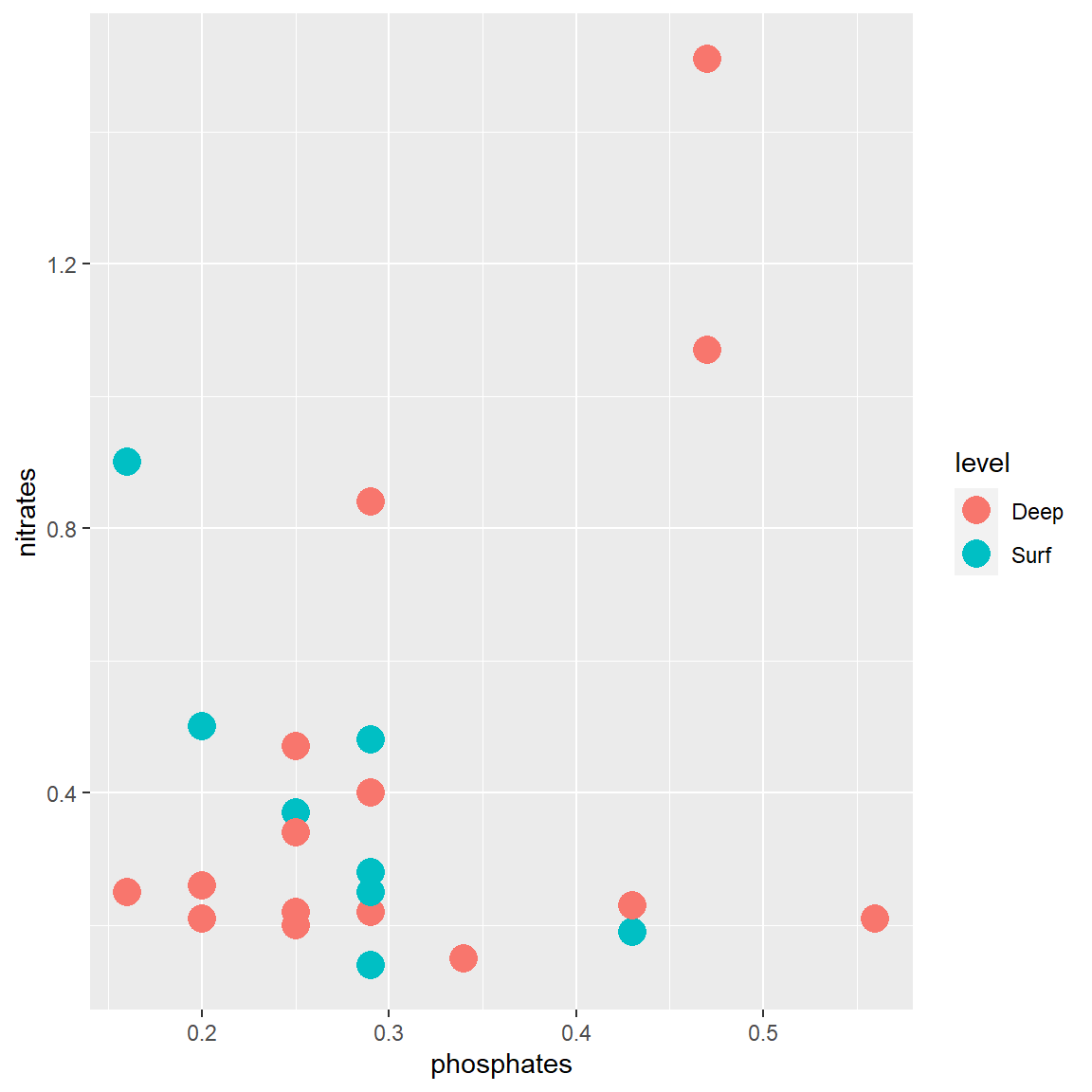
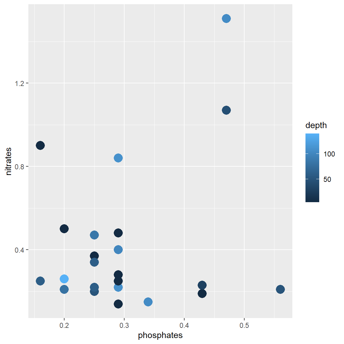
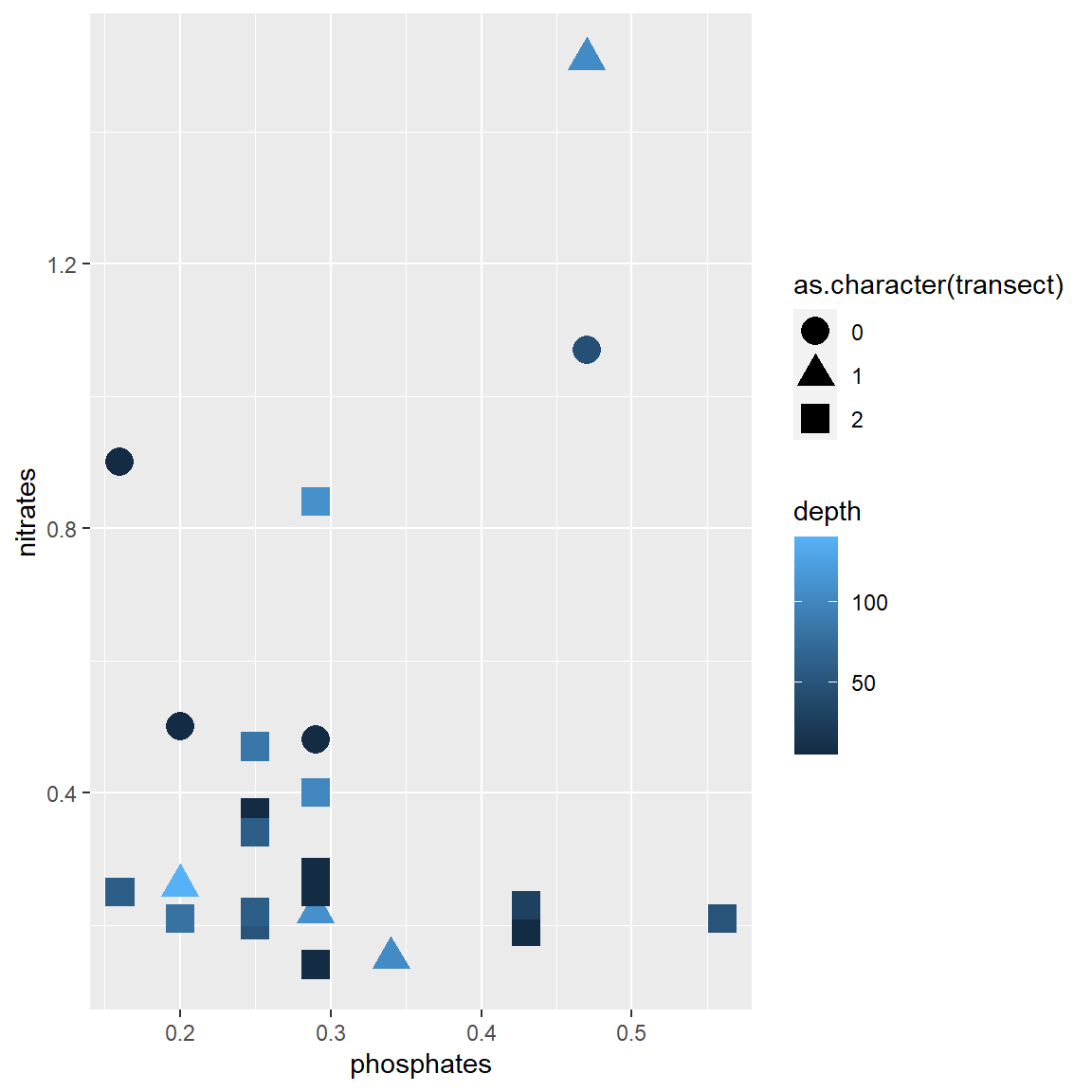
Color according to depth (continuous)

The mapping aesthetics must be an argument of the aes function
Add: color=depth

 ggplot(samples,
        aes(x=phosphates, 
            y=nitrates,
            color=depth)) + 
  geom_point(size=5)

Symbol according to transect (continuous)

Add: shape=transect

 ggplot(samples,
        aes(x=phosphates, 
            y=nitrates,
            color=depth,
            shape=transect)) + 
  geom_point(size=5)

Error in `geom_point()`:
! Problem while computing aesthetics.
ℹ Error occurred in the 1st layer.
Caused by error in `scale_f()`:
! A continuous variable cannot be mapped to the shape aesthetic
ℹ choose a different aesthetic or use `scale_shape_binned()`

Symbol according to transect (continuous)

Add: shape=as.character(transect)

 ggplot(samples,
        aes(x=phosphates, 
            y=nitrates,
            color=depth,
            shape=as.character(transect))) + 
  geom_point(size=5)

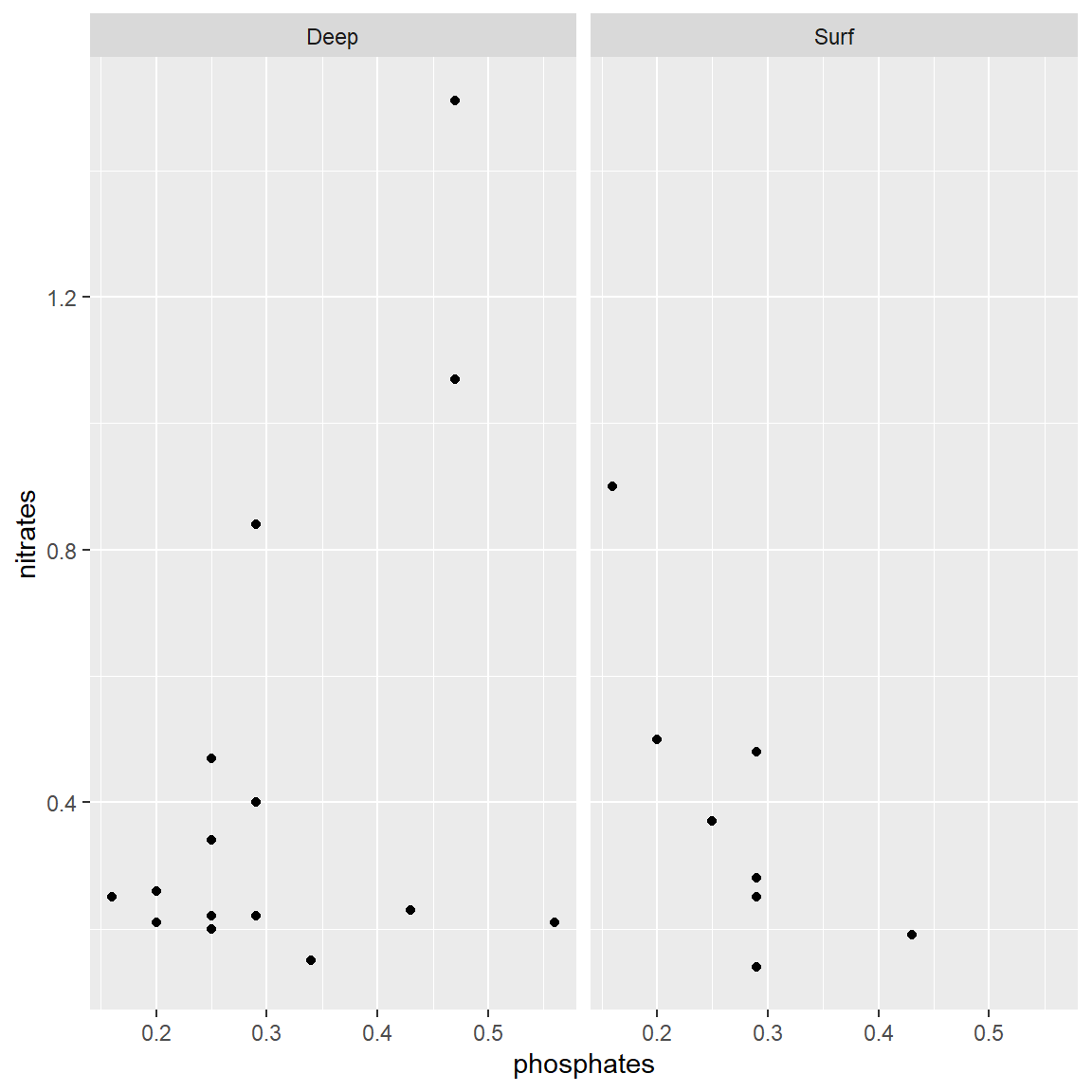
Panels depending on one variable

 ggplot(samples,
        aes(x=phosphates, 
            y=nitrates)) +
  geom_point() +
  facet_wrap(~ level)

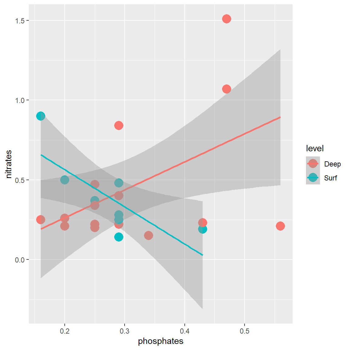
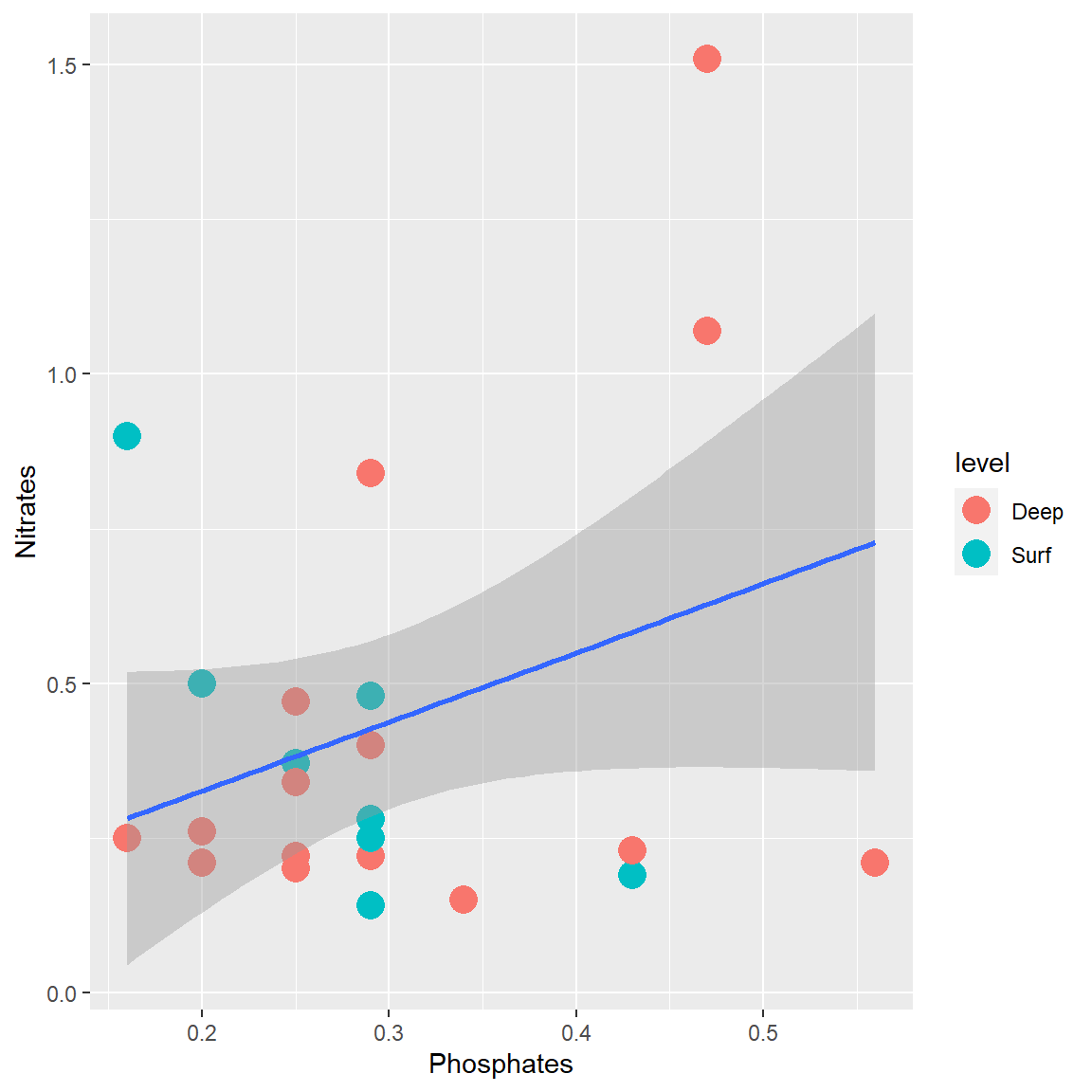
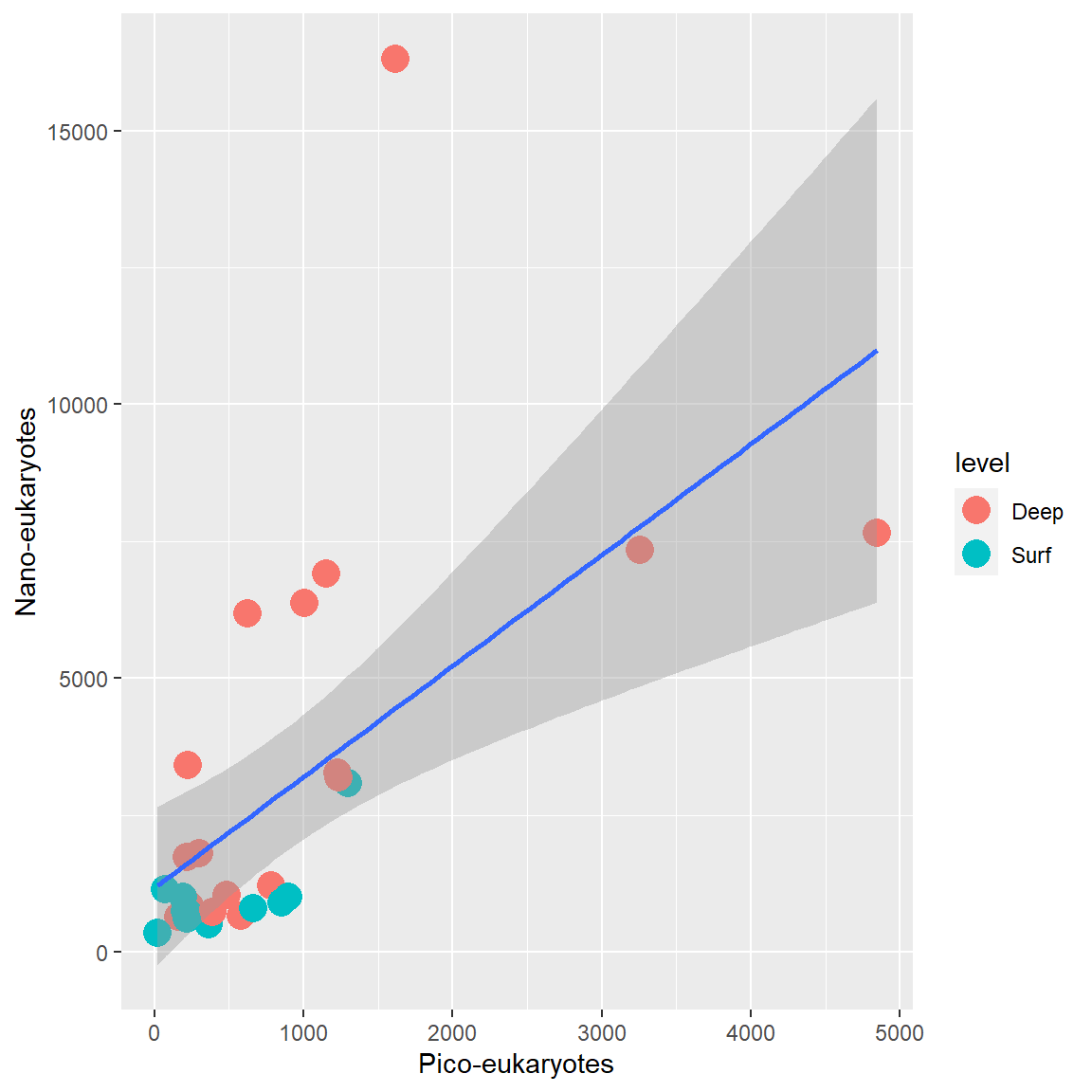
Adding a regression line

Add: geom_smooth()
You can choose the type of smoothing “lm” is for linear model

 ggplot(samples,
        aes(x=phosphates, 
            y=nitrates, 
            color=level)) +
  geom_point(size=5) +
  geom_smooth(mapping = aes(x=phosphates, 
                            y=nitrates), 
              method="lm")

Adding a regression line

If the mapping is in the ggplot function is for all the geom….

 ggplot(samples,
        aes(x=phosphates, 
            y=nitrates)) +
  geom_point(aes(color=level), 
             size=5) +
  geom_smooth(mapping = aes(x=phosphates, 
                            y=nitrates), 
              method="lm")

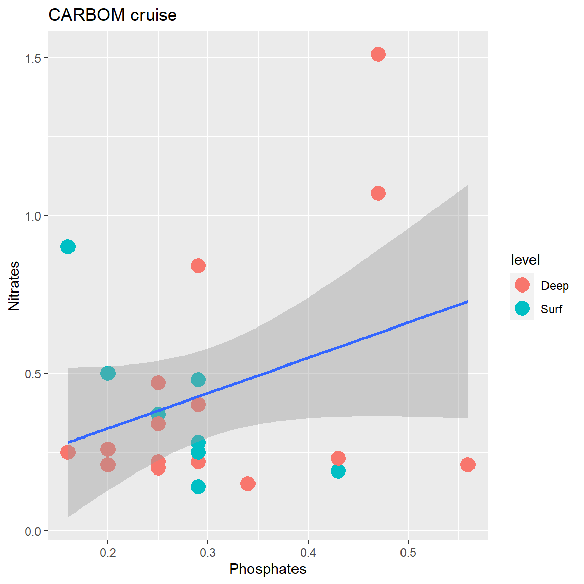
Finalizing the graph

Adding labels and legends

 ggplot(samples) + 
  geom_point(mapping = aes(x=phosphates, 
                           y=nitrates,
                           color=level), 
             size=5) +
  geom_smooth(mapping = aes(x=phosphates, 
                            y=nitrates), 
              method="lm") +
  xlab("Phosphates") + 
  ylab("Nitrates") + 
  ggtitle("CARBOM cruise")

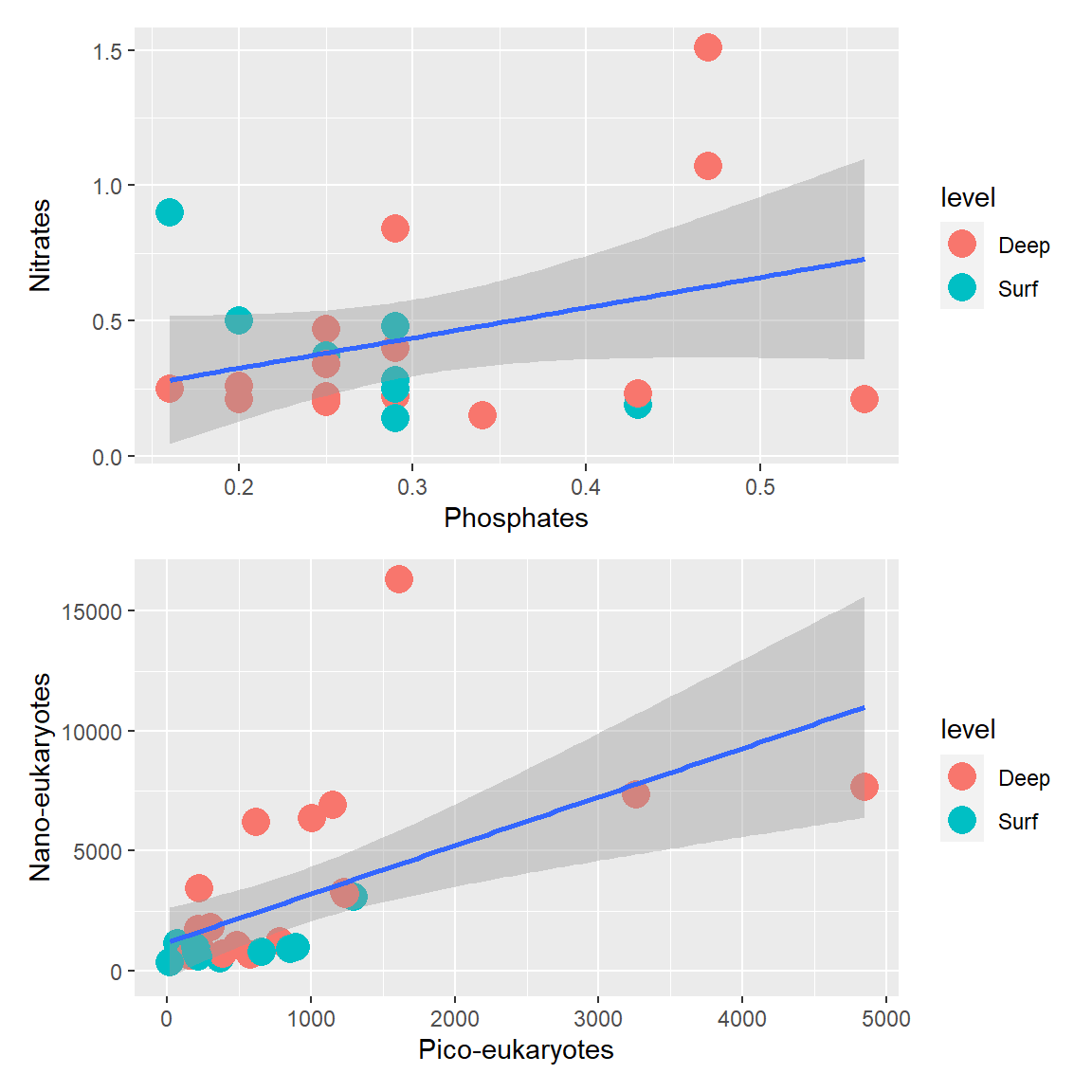
Multigraphs (patchwork package)

First graph

 g1 <- ggplot(samples) + 
  geom_point(mapping = aes(x=phosphates, 
                           y=nitrates,color=
                             level), size=5) +
  geom_smooth(mapping = aes(x=phosphates, 
                            y=nitrates), 
              method="lm") +
  xlab("Phosphates") + 
  ylab("Nitrates")

 g1

Second graph

 g2<- ggplot(samples) + 
  geom_point(mapping = aes(x=nanoeuks, 
                           y=picoeuks,
                           color=level), 
             size=5) +
  geom_smooth(mapping = aes(nanoeuks, 
                            y=picoeuks), 
              method="lm") +
  xlab("Pico-eukaryotes") + 
  ylab("Nano-eukaryotes") 

 g2

Package patchwork

Other packages:
- gridExtra
- cowplot

library(patchwork)
(g1 / g2)

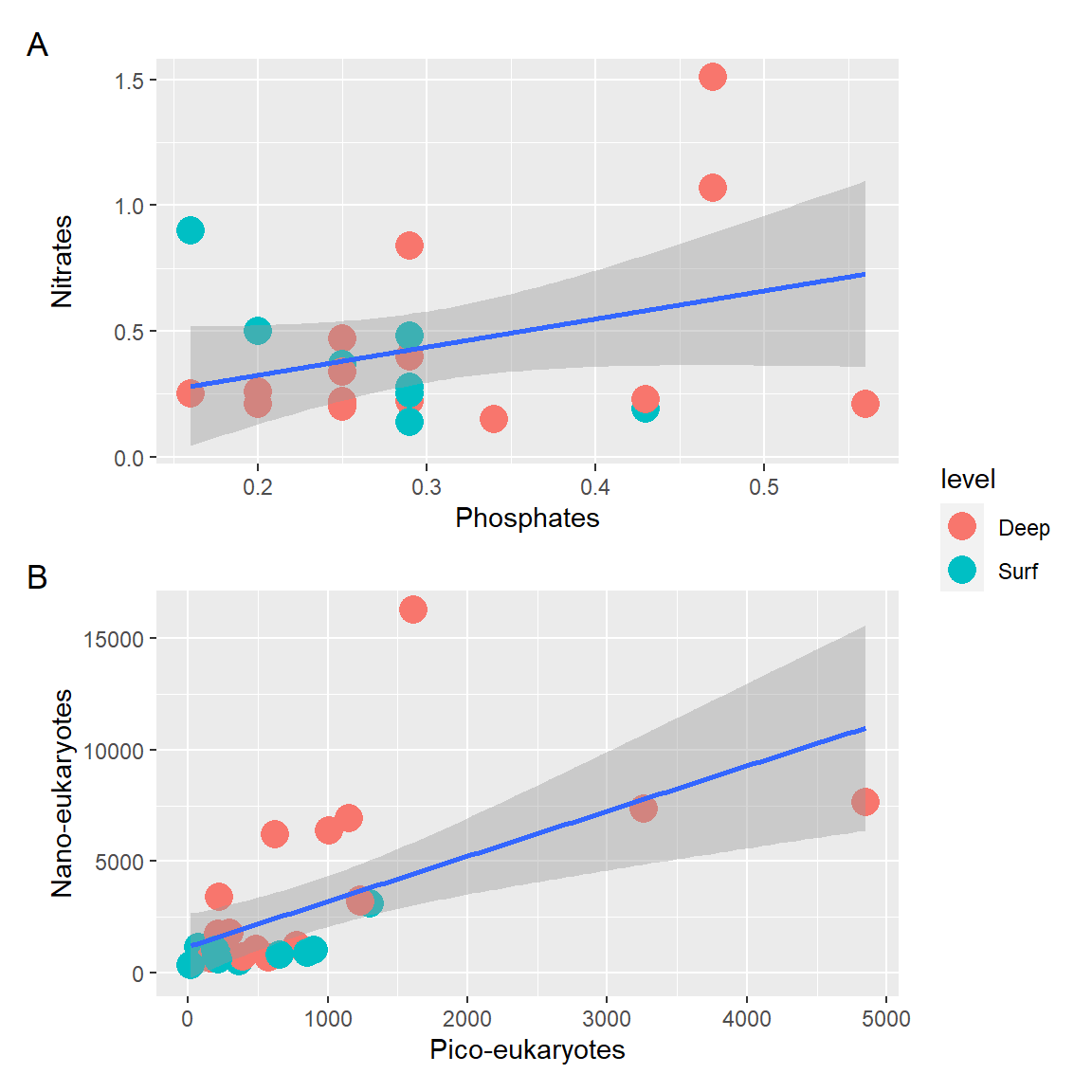
Package patchwork

Adding annotation
Collecting legends

g1 / g2 +
  plot_annotation(tag_levels = 'A') +
  plot_layout(guides = 'collect')

Package esquisse

ggplot2 syntax

Anatomy of a plot

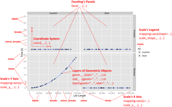
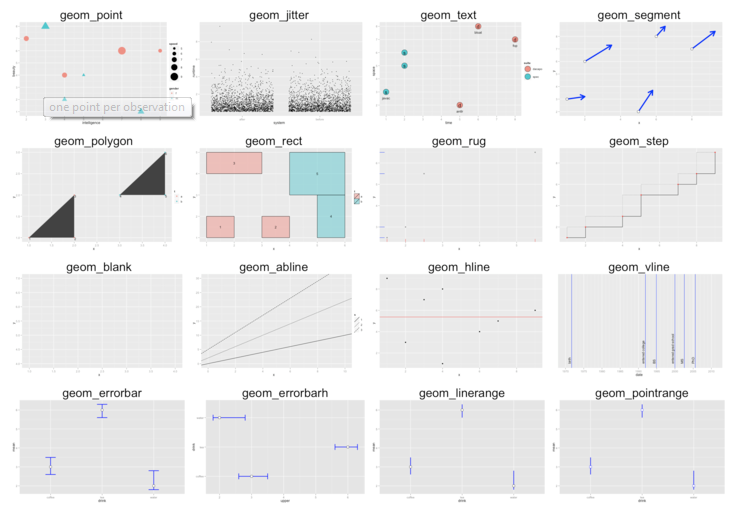
Geometries

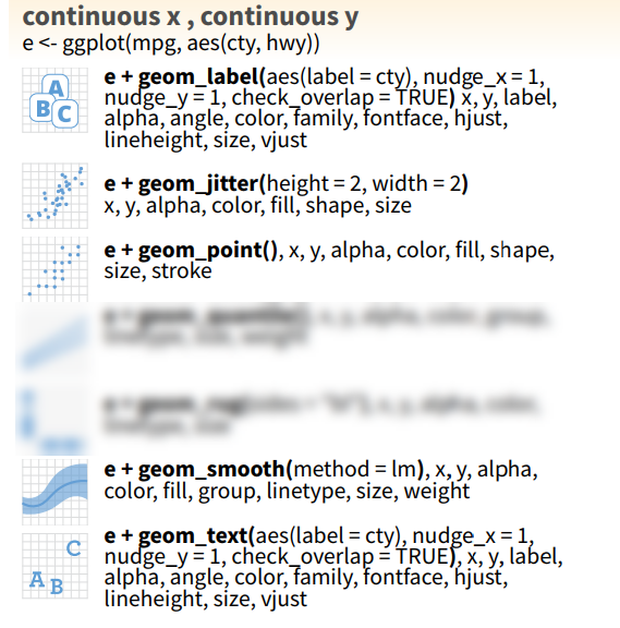
Continuous x and y

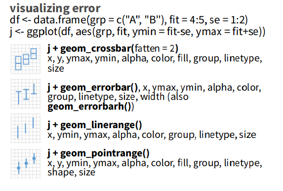
Plotting error

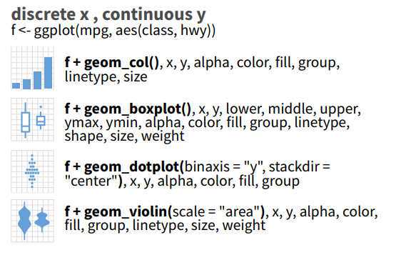
Discrete x - Continuous y

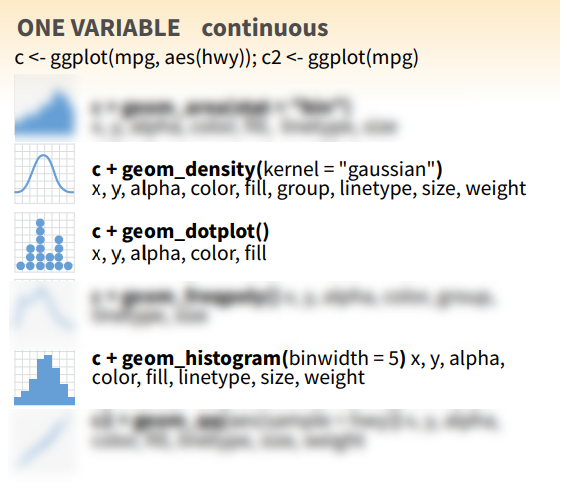
Continuous x

3D

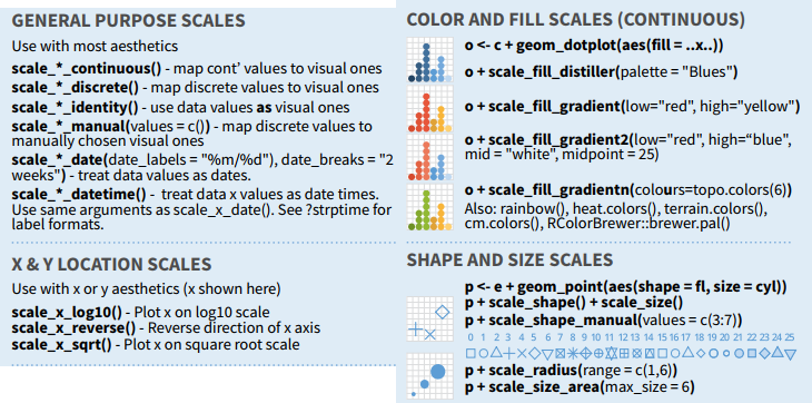
Modifying axis and scales

Palettes

Package tmaptools
- Function : palette_explorer()
Package paletteer
- More than 1000 palettes

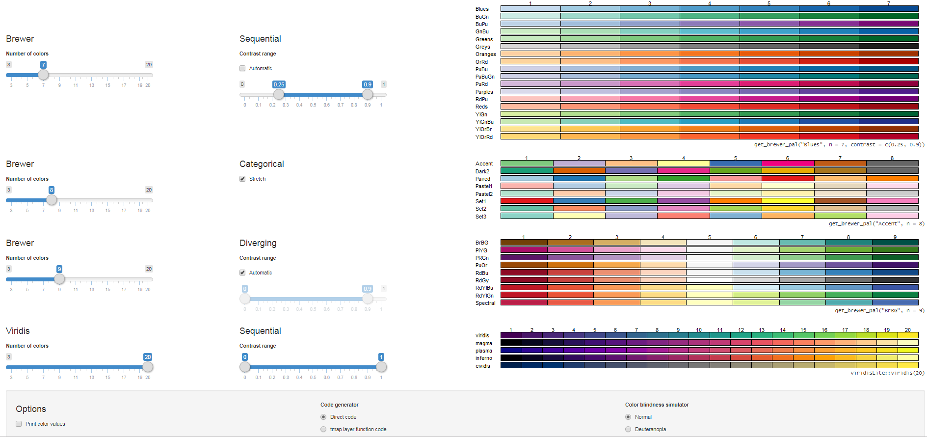
Palettes

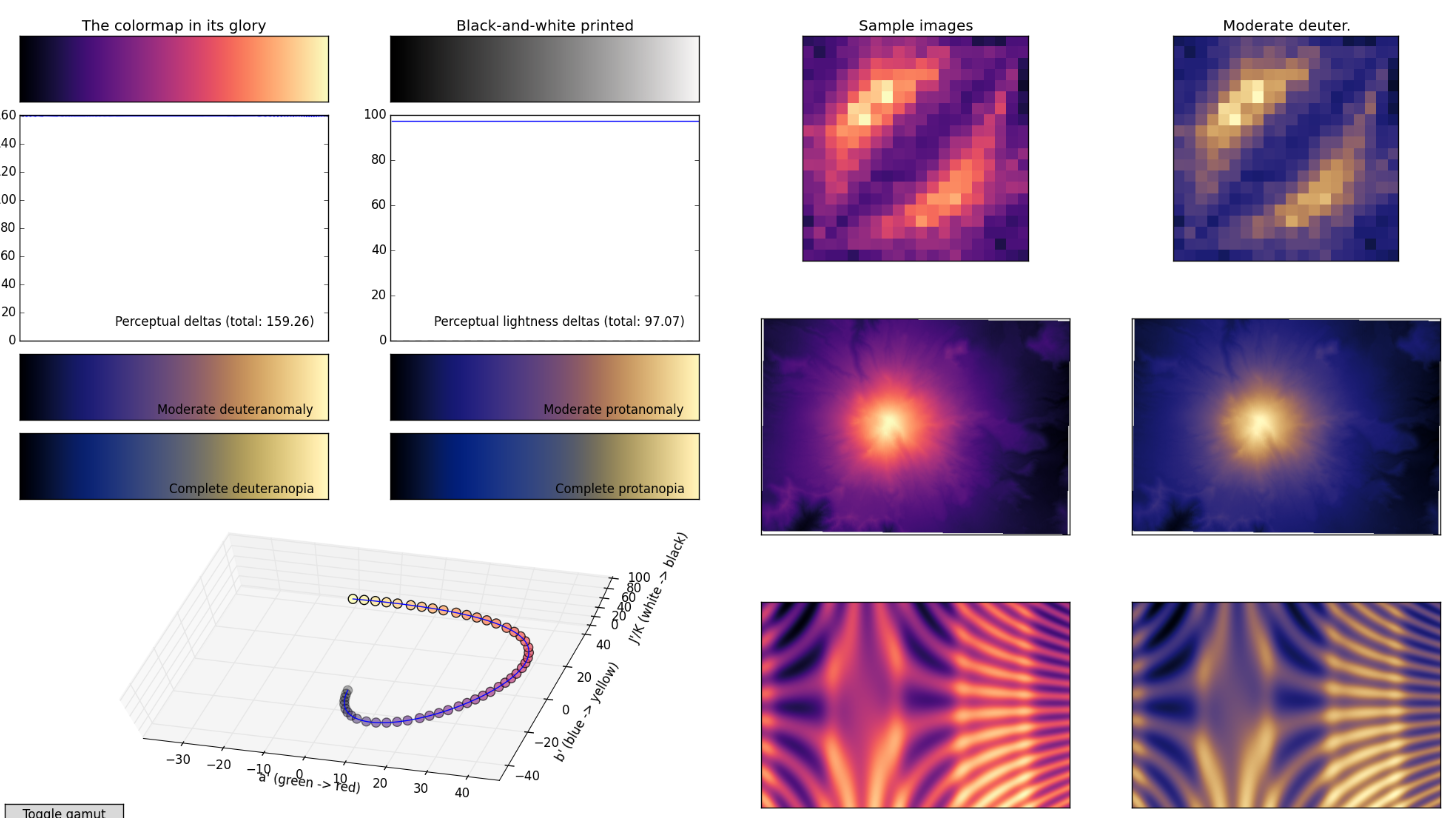
Use color blind friendly palettes
- viridis (e.g. scale_colour_viridis_c())

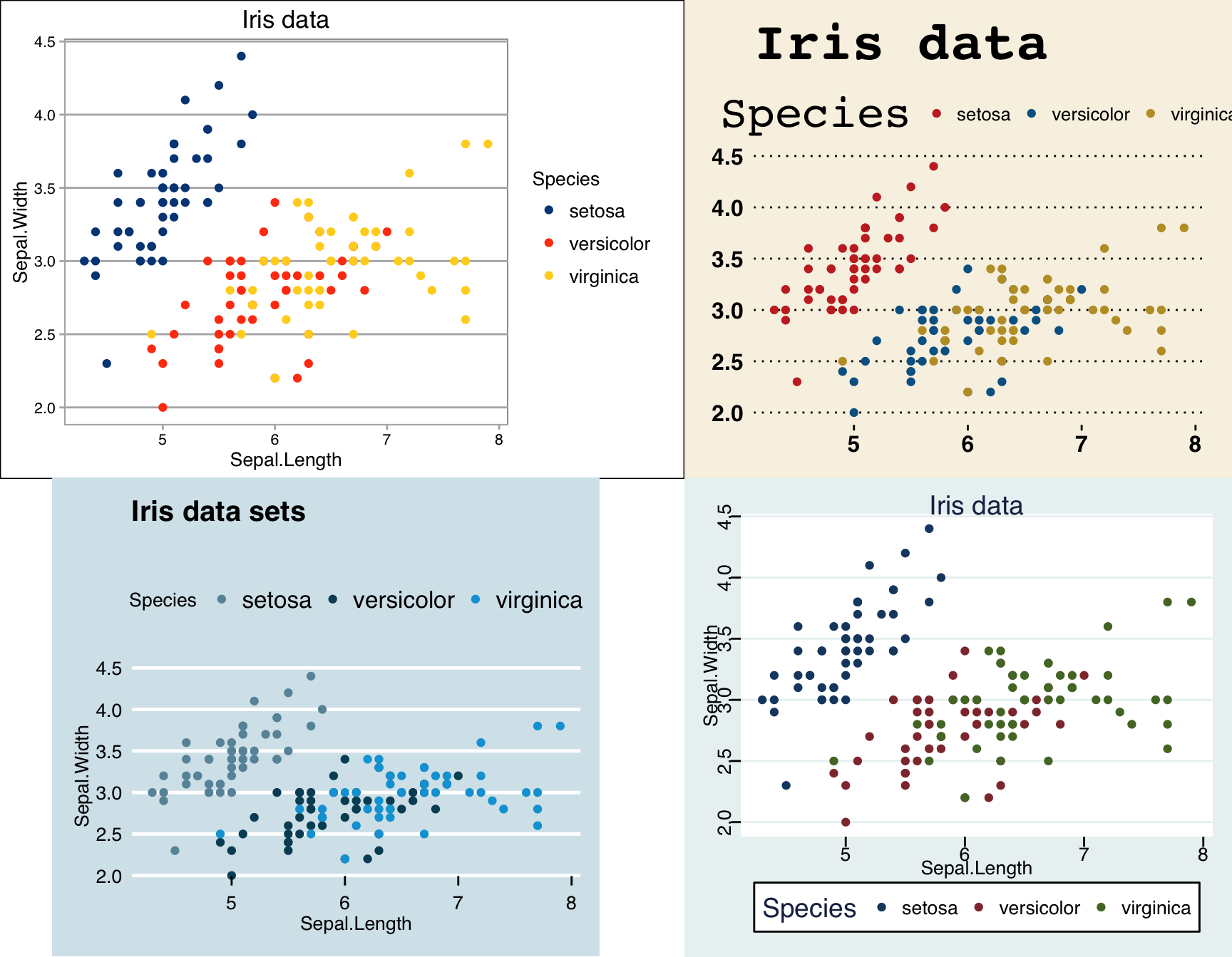
Themes

Extensions

Let’s do a graph

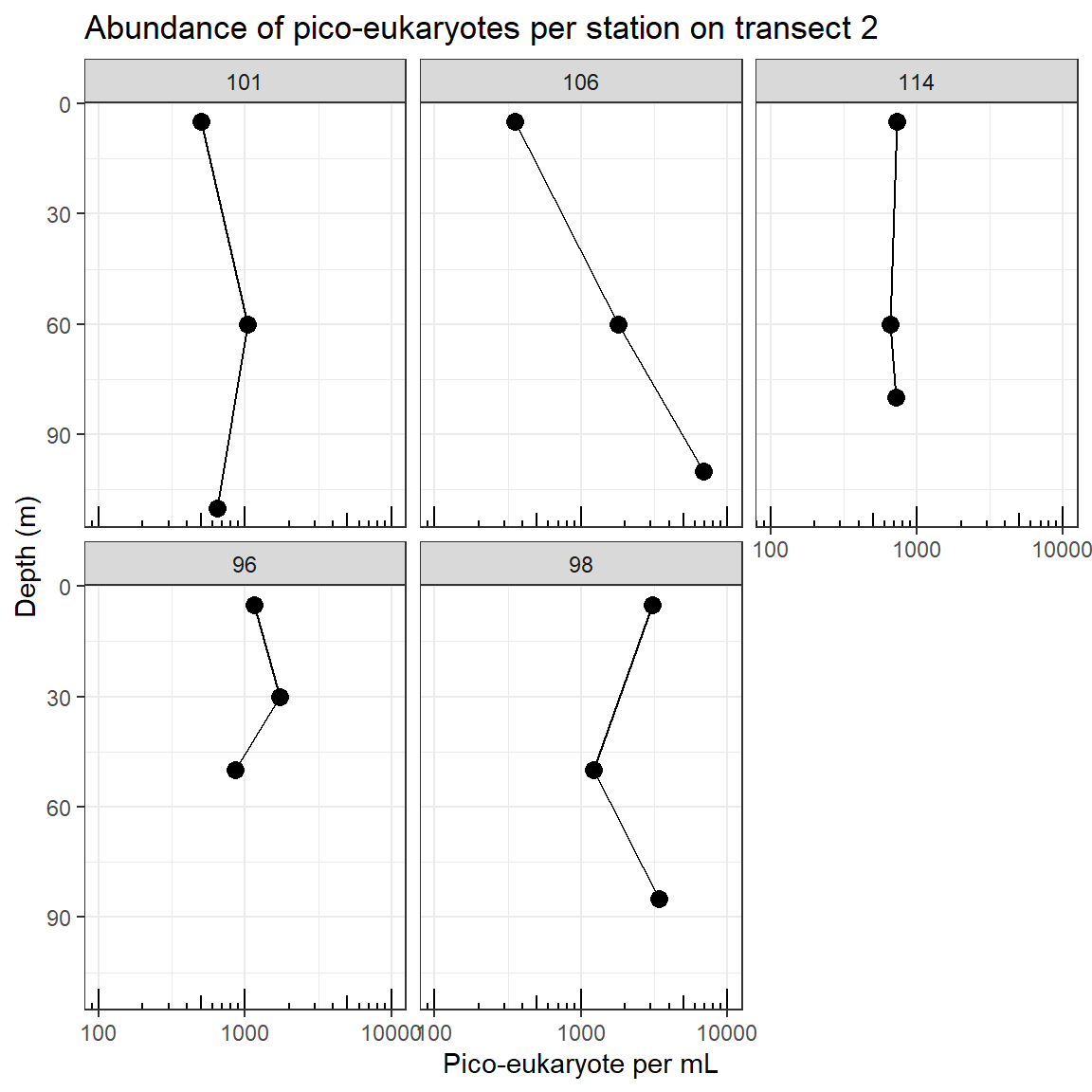
Your mission

Reproduce graph on right

Only transect 2
One panel per station
Increasing depth
Log scale for x
White background

Instructions

Work by group of 2 (1 expert, 1 less expert)
Send code and results by element.io by private message to Daniel
Do not search Internet for precise solution

Recap

Conceptualize your graph before coding
Decide what element is fixed and what varies
It takes time to get what you want…
Exploratory vs. final

Next time: Markdown and Quarto